2019 International Conference on Information Technology, Electrical and Electronic Engineering (ITEEE 2019) ISBN: 978-1-60595-606-0
The Comparison of Two Empirical Runoff Yield Models and
Three Physical Models
Kai-wen WANG
1and Xiao-hua YANG
2,*1
Key Laboratory of Water Cycle and related Land Surface Processes, Institute of Geographic Sciences and Natural Resources Research, Chinese Academy of Sciences, Beijing 100101, China
2,*
State Key Laboratory of Water Environment Simulation, School of Environment, Beijing Normal University, No. 19, XinJieKouWai St., HaiDian District, Beijing 100875, China
*Corresponding author
Keywords: Empirical infiltration model, Physical infiltration model, Runoff yield calculation.
Abstract. We used the particle swarm optimization algorithm to make comparisons between five
two-parameter runoff models, two empirical models, LCM and SCS; and three physical models, GA, GAML and GAF, in calculating rainfall-runoff yield. The comparison results show that the qualified rate and coefficient of determination of the LCM, SCS, and GAF models were higher than 83% and 0.89, respectively. GA and GAML models can simulate the mean value of data; however, they performed poorly in describing the relationship between rainfall and runoff yield. The qualified rate and coefficient of determination of the GA and GAML models were lower than 50% and 0.50, respectively. In conclusion, LCM and SCS models can be used to calculate the runoff yield of small ungauged watersheds. Small watersheds with gauged data can use GAF model, which has high accuracy and physically meaningful parameters, to calculate runoff yield.
Introduction
Rainfall-runoff is a key component of hydrological cycles, and short-duration high-intensity rainfall often causes floods; thus, modeling the runoff process for individual floods is important in many water resource problems [1]. A great amount of rainfall-runoff models have been developed and can be divided into three categories: empirical, conceptual, and physically based models.
During the period of 1958-1978, Liu et al. [2] conducted a series of artificial rainfall experiments in the field at many locations in China, and established an empirical equation (i.e., LCM) to calculate the infiltration losses during the runoff period. Based on the LCM model, coupled with other hydrological models, some distributed hydrological models were built, e.g., HIMS and EcoHAT, which performed well in calculating catchments under different conditions in China, Australia, and some parts of America [3,4]. Around the same time, the United States Department of Agriculture developed the SCS model [5], which has been improved since then. This model has been widely used for different catchments, basins, and watersheds around the world [6], and has also been used in famous hydrological models, such as SWAT, EPIC, and AGNPS. Among the various rainfall-runoff models in the literature, the Green–Ampt model [7] is the first physically based equation describing the infiltration of water into the soil. Developing over a century, the GA model continues to develop. The GA model and its improved versions have been widely used in infiltration and runoff calculations [8-10], such as the LISEM, WEPP, and SWAT models. The GA model is based on the assumption that soil may be regarded as a bundle of tiny capillary tubes irregular in area, direction, and shape. Mein and Larson [11] demonstrated the application of the GA equation for the conditions of constant rainfall intensity. Using the initial abstraction as a basic parameter, Li [12] acquired the GAF infiltration equation during the runoff period, which solved the problem of estimating the capillary pressure head at the wetting front.
at different spatial and temporal scales [13, 14]. In recent years, some researchers have compared models containing diverse mathematical and physical mechanisms. Chahinian et al. [15] compared the GA and SCS models in simulating event-based rainfall at the field scale and found the GA model and its improved versions have high accuracy. Nearing et al. [16] built an empirical relationship between the effective conductivity of GA and CN in SCS. Tested by experiments, the empirical relationship performed better in runoff calculations than SCS. Using theoretical analyses and numerical simulations, Li et al. [12] found that the SCS model is a simple linear representation of the LCM model and that the LCM model reflects more significantly the nonlinearity of catchment runoff. Li et al. [17] developed a complete governing equation (i.e., GAF) for rainfall infiltration based on the Green-Ampt assumption. The initial abstraction, which was calculated using the SCS-CN method, was used as a basic parameter in the GAF model. By theoretical analysis, the LCM and SCS models were united using the GAF model, and its analytical solution was characterized by power-exponential and reciprocal linearity features. Grimaldi et al. [18, 19] established the CN4GA rainfall-runoff model for small and ungauged basins, which was a combination of the SCS and GA models. Validation results indicated that the CN4GA model provided more realistic results than the SCS method.
The comparison of the effects of simulating at different scales and mechanisms has been made, but the comparison of physical models needs precise soil physical parameters. The objective of this paper is to make the comparison of two empirical runoff yield models and three physical models in rainfall-runoff calculations. Considering the difficulties in acquiring soil physical parameters and in their spatial heterogeneity, we used the Particle Swarm Optimization (PSO) algorithm to optimize the parameters.
Model
LCM Model
In the LCM model, the relationship between infiltration losses and rainfall is quantified as:
1
=
i R P (1)
where i is the average intensity of the losses of rainfall during the runoff period, 𝑃̅ is the average
rainfall intensity, R is the coefficient of losses related to the soil type or soil flow properties, and γ1
is the index of the losses.
SCS Model
Based on the water balance equation and two hypotheses, the losses of rainfall is described by the famous SCS model as:
1 1 1
a
F S PI (2)
where F is the actual infiltration losses, S is the potential maximum retention after runoff occurs,
and Ia is the initial abstraction.
S and Ia can be estimated by the curve number (0≤CN≤1000):
25400
254 , a
S I S
CN
(3)
According to a large number of experiments, λ=0.2 is widely used by the Soil Conservation
GA & GAML Models
The GA model assumes that the wetting front infiltrating into a semi-infinite, homogeneous soil at uniform initial water content occurs as a saturated pulse. Considering stable rainfall intensity, it was extended for non-immediate ponding by Mein and Larson and referred to as the GAML model. Both models are under a constant positive pressure head and have wetting fronts driven by a constant capillary pressure. If the vertical z-axis is positive downward, the implicit equations of the GA and GAML models during the runoff period are:
s
s
( ) ln(1 )
( )
s f i
f i
F
K t F s
s (4)
s s s s s( ) ln( )
( ) ( )
( ) ln(1 ) ( )
f i
f i s f i s
f i s
f i s s s
P s
s K s
F P K
F s K t
s P P K P K K
(5)
where Ks is the soil saturated hydraulic conductivity, F(t) is the infiltration during the runoff period,
θsis the saturated volumetric water content, and θi is the initial volumetric water content.
GAF Model
The implicit form of the GAF model during the runoff period is:
0
s a a
dF
K F P I I F
dt
(6)
where t=0 when runoff begins and dF/dt=P. Using the Lambert W function, the explicit form of
GAF is:
s exp s2
a
s s s s s a
P K P P P P K t
F t I W
K K K P K P K P PI
(7)
Where W is the Lambert W function.
Evaluation Indexes of Models
As performance measures, we selected the relative percent error between the observed and
simulated total infiltration losses for rainfall Err and the Nash and Sutcliffe index NS. These
statistics are expressed by the following relationships:
1
1
( ) 100
n m o i rr n o i F F E F (8) 2 2 , ( ) 1 ( ) o m
o o mean
F F NS F F
(9)where Fm and Fo are the observed and modeled infiltration losses of rainfall, respectively, and
Fo,mean is the mean value of the observed infiltration losses of rainfall.
predicted events and total rainfall events to calculate the qualified rate of each model. Model
qualified rates and NS indexes are shown in table 1.
As seen in table 1, the GAML model greatly underestimated the infiltration losses, and by
comparing NS indexes and qualified rates, the LCM, SCS, and GAF models have higher accuracy,
[image:4.595.61.532.162.237.2]whereas the GA and GAML models can simulate only less than half of the data accurately.
Table 1. The qualified rate and NS Index for each model.
LCM SCS GA GAML GAF
Err (Qualified
rate)
NS
Err (Qualified
rate)
NS
Err (Qualified
rate)
NS
Err (Qualified
rate)
NS
Err (Qualified
rate)
NS
0.38
(84.2) 0.89
0.04
(86.9) 0.90
-1.74
(47.4) 0.41
-44.45
(42.1) 0.05
3.24
(84.2) 0.91
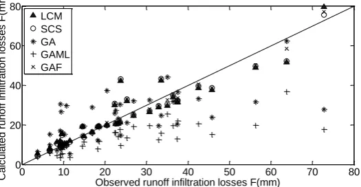
The scatter plot of calculated and observed runoff infiltration losses for all five models is shown in Fig. 1. Results for the GA model are concentrated near the average, which does not reflect the relationship between rainfall and runoff. The GAML model can simulate the runoff field for small amounts of rainfall, but seriously underestimated runoff for rainfall greater than 20 mm, thus the GAML model does not reflect the rainfall-runoff data accurately. The LCM, SCS, and GAF models demonstrate accurate results and are less affected by error points.
Figure 1. Comparison of calculated and observed runoff for the 5 models.
Conclusion
Model selection for flood estimation is usually subjective. To choose models suitable for rainfall-runoff calculations, we use rainfall runoff data from bare soil plots and compare five different models. The PSO algorithm is used to optimize the different equations. The results show that the qualified rate and NS index of the LCM, SCS, and GAF models are higher than 83% and 0.89, respectively. These models accurately simulate the relationship between rainfall and runoff yield. The GA and GAML explicit models with the Lambert W function can simulate the mean of the data; however, they perform poorly in describing the relationship between rainfall and runoff yield. The qualified rate and NS index of the GA and GAML models are lower than 50% and 0.50, respectively. Therefore, LCM and SCS models can be used to calculate the runoff yield of small ungauged watersheds. Small watersheds with gauged data can use GAF model, which has high accuracy and physically meaningful parameters, to calculate runoff yield.
Acknowledgement
This work was supported by the Project of National Natural Foundation of China (No. 51679007), the National Key Research Program of China (No. 2017YFC0506603), and the State Key Program of National Natural Science of China (No. 41530635).
0 10 20 30 40 50 60 70 80
0 20 40 60 80
Observed runoff infiltration losses F(mm)
C
a
lc
u
la
te
d
ru
n
o
ff
i
n
fi
lt
ra
ti
o
n
l
o
s
s
e
s
F
(m
m
)
[image:4.595.183.446.330.466.2]References
[1] K. Wang, X. Yang, X. Liu, & C. Liu, A simple analytical infiltration model for short-duration rainfall, Journal of Hydrology. 555(2017), 141-154.
[2] C. Liu, & G. Wang, The estimation of small-watershed peak flows in China, Water Resources Research, 16(1980), 881-886.
[3] J. Li, C. Liu, Z. Wang, & K. Liang, Two universal runoff yield models: SCS vs. LCM, Journal of Geographical Sciences. 25(2015), 311-318.
[4] Y. J. Wang, S. D. Wang, S. T. Yang, et al., Dynamic Simulation of Vegetation Eco-water of the Yellow River Basin, Journal of Natural Resources. 29(2014):431-440.
[5] SCS, Hydrology, National Engineering Handbook, Supplement A, Section 4 Chapter 4, Soil Conservation Service, Washington, DC: USDA. 1985.
[6] J.F. Liu, W.G. Jiang, W.F. Zhan et al., Processes of SCS model for hydrological simulation: a review, Research of soil and water conservation. 17(2010):120-124. (In Chinese)
[7] W. Green & G. Ampt, Studies on soil physics part I: the flow of air and water through soils, Journal of Agricultural Science. 4(1911), 1-24.
[8] R. Kabiri, A. Cha, & R. Ba, Comparison of scs and green-ampt methods in surface runoff-flooding simulation for klang watershed in Malaysia, Open Journal of Modern Hydrology. 3(2013), 102-114.
[9] K. W. King, J. G. Arnold, & R. L. Bingner, Comparison of Green-Ampt and curve number methods on Goodwin Creek watershed using SWAT, Transactions of the ASAE. 42(1999): 919-925.
[10] J. A. Van Mullem, Runoff and peak discharges using Green-Ampt infiltration model, Journal of Hydraulic Engineering. 117(1991): 354-370.
[11] R. G. Mein, & C.L. Larson, Modeling the infiltration component of the rainfall-runoff process. WRRC Bull. 43, Water Resources Research Center, University of Minnesota, Minneapolis. 1971.
[12] J.Li, Study the mechanism of runoff generation and flow routing processes in semi-arid sub-humid regions, Beijing: The university of Chinese Academy of Sciences, Institute of Geographic Sciences and Natural Resources Research. 2015. (In Chinese)
[13] K. M. Loague, & R. A. Freeze, A comparison of rainfall runoff modeling techniques on small upland catchments, Water Resources Research. 21(1985): 229-248.
[14] S. Mishra, J. Tyagi, V. Singh, Comparison of infiltration models, Hydrological Processes. 17 (2003), 2629-2652.
[15] N. Chahinian, R. Moussa, P. Andrieux, & M. Voltz, Comparison of infiltration models to simulate flood events at the field scale, Journal of Hydrology. 306(2005), 191-214.
[16] Nearing M A, Liu B Y, Risse L M, et al., Curve Numbers and Green-Ampt Effective Hydraulic Conductivities, JAWRA Journal of the American Water Resources Association. 32(1996): 125-136.
[17] J. Li, Z. Wang, & C. Liu, A combined rainfall infiltration model based on Green-Ampt and SCS-Curve Number, Hydrological Processes. 29(2014), 2628-2634.
[18] S. Grimaldi, A. Petroselli, & N. Romano, Green-ampt curve-number mixed procedure as an empirical tool for rainfall–runoff modelling in small and ungauged basins, Hydrological Processes. 27(2013a), 1253-1264.