Optimizing Empty Container Relocation Plans for Marine Transportation

2019 International Conference on Artificial Intelligence, Control and Automation Engineering (AICAE 2019) ISBN: 978-1-60595-643-5

Optimizing Empty Container Relocation Plans for Marine Transportation

Kenji Tanaka

, Yuki Kimura

and Jing ZHANG

1_{Department of Systems Innovation, The University of Tokyo, Tokyo, Japan}

2_{School of Mathematics, Physics and Information Science, Zhejiang Ocean University, China}

*Corresponding author

Keyword: Marine logistics, Empty Container, Imbalance, Simulation, Method.

Abstract. Due to the structure of global supply chains, there is an imbalance in trade between East Asia and the rest of the world. As a result, many empty containers are generated in the North American, European, and Asian ocean transportation routes. Focusing on this problem, in this paper we formulate a reallocation plan for empty containers in a maritime container logistics network connecting multiple bases, and minimize the relocation cost. We also use actual data from shipping companies to quantify and verify the cost reduction effect in a maritime shipping alliance from the viewpoint of the cost of relocating empty containers, and show the effectiveness and practicality of our proposed method.

Introduction

With globalization of the world’s economy, international maritime transport is becoming increasingly popular [1]. Container transport is attracting particular attention, with cargo volumes increasing almost fivefold from 1995 to 2016.

The global supply chain is configured to carry goods manufactured in East Asia to locations throughout the world. As a result, container transport has become active and there is an imbalance in the directionality of container travel. There are container shortages in East Asia, especially in China, because exports exceed imports. Surplus containers accumulate in ports with an excess of imports. That is, while there are some ports with room to stack empty containers, there are other ports with no room. It therefore becomes necessary to circulate and rearrange empty stacked containers on surplus land.

As an existing approach to this problem, Song et al. classified empty container relocation into three groups. The first focuses on empty container transport in a maritime container logistics network. The second considers inland container transport networks or empty container transport in integrated transport including inland transport. The third incorporates decision-making problems. We studied empty container transport as a constraint. Song et al also used dynamic programming to consider uncertain demands and to establish an optimal inventory management method that is responsive to acceptable shortage rates [1–5]. Zheng et al. found optimal combinations of ports with supply and demand for empty containers in a maritime container network by reducing the assignment problem in multiple ports [6–9].

For such existing research, the scope is limited to networks such as hubs and spokes, and requires deciding the number of containers to be exchanged between ports. Further, these methods do not consider shipping schedules or inventory management of container vessels, and do not adopt a time axis [10–11].

container inventory shortage rates to below a certain level depending on the supply and demand of empty containers at each port. In addition, verification is performed using actual data obtained as part of industry-academia collaboration involving shipping companies, and the academic and practical values of the proposed method are shown.

Model Approach

Modeling and Entities

Under the constraint that the empty container shortage rate at each port remains below a certain level, let the objective function be cost minimization for empty container relocation. Furthermore, the optimal allocation of empty containers must consider port space and container vessels. The following entities are in this model:

 Shipping company: A company engaged in the shipping business. The objective function minimizes the cost of empty container transport.

 Harbor: A company involved in port management. We assume that terminal operation costs, including terminal facility costs, are paid to the port carrier.

 Container leasing company: In addition to shipping company ownership, we also consider containers owned by container leasing companies.

 Container manufacturing company: Shippers tend to prefer new containers. Shipping and leasing companies aim to improve quality of service over minimizing container age, but this study does not consider the manufacture and disposal of containers.

 Cargo owner: Cargo owners are customers requesting ocean transportation. We consider cargo owners as consumers of empty containers.

Demand Forecasting for Empty Containers

First, we define empty container demand. As a premise, the occurrence of empty containers in ports is considered as “production,” and “consumption” is when goods are loaded on empty containers. Empty containers are considered as stock until loading. Because empty containers are “consumed” when transport demand occurs, the number of inventory changes in each port is the number of empty containers returned minus the number of empty containers transported from the port. Here, the empty container demand is the same value as the decrease in empty container stock. In a given port (p), empty container demand 𝐷𝑒𝑚𝑎𝑛𝑑_𝑝,𝑑 in a certain period (d) is calculated using the transport demand 𝑇𝑟𝑎𝑛𝑠𝑝𝑜𝑟𝑡𝑝,𝑑 and the number of empty container returns 𝑅𝑒𝑡𝑢𝑟𝑛𝑝,𝑑, expressed

as a formula. As mentioned above, the manufacture and disposal of empty containers are not considered.

𝑫𝒆𝒎𝒂𝒏𝒅_𝒑,𝒅= 𝑻𝒓𝒂𝒏𝒔𝒑𝒐𝒓𝒕_𝒑,𝒅− 𝑹𝒆𝒕𝒖𝒓𝒏_𝒑,𝒅 (1) 𝑇𝑟𝑎𝑛𝑠𝑝𝑜𝑟𝑡𝑝,𝑑 : Empty container consumed (transportation demand)

𝑹𝒆𝒕𝒖𝒓𝒏_𝒑,𝒅 : Empty container refilled (stock replenishment)

Empty Container Inventory

Containers have economic value because they are used for marine logistics and generate profits. There are idle periods where they are not used for transport or at ports, and during that period they can be regarded as inventory that does not generate profits. The main objective of inventory management is to minimize total costs. There are various factors related to the cost of inventory control, but in this study, we mainly classify three.

 Inventory maintenance cost: A general term for expenses such as location costs, maintenance costs, and insurance premiums that arise per unit of inventory. In this study, we consider the cost per day of one empty container.

fixed number of empty containers. Therefore, unlike a general product, the cost of entering ports is not incurred every time an order is placed.

 Out-of-stock costs: For empty container shortages, we formulate a plan under the constraint that the shortage rate in each port must be kept below a certain level.

Empty Container Flexibility and Inventory

The ordering system mainly includes a quantitative ordering point system and a regular ordering point system. The former is for placing a fixed order volume when the order interval is not fixed. The latter places periodic orders at different quantities. Considering the ordering method for empty container inventory, the interval of the ordering period of the empty container inventory at each port is determined by the schedule of the container ship calling on port.

In this study, on the premise of fixed-day service, the number of container ships determines the travel schedule. For example, assume it takes 21 days to complete a route and three container vessels will provide fixed-day service. In this case, one container ship will arrive each week. The amount of accommodation between a port 𝑝 ∈ 𝑃 and a container ship 𝑙 ∈ 𝐿 is defined as 𝑥_𝑙,𝑝 as in Equation 2, and takes a positive or negative integer value. 𝑥𝑙,𝑝 assumes positive values when an

empty container is transferred from a container ship to a port. As a result, it is possible to formulate the amount of interchange without distinguishing between supply or demand ports. Even in the same port, since 𝑥_𝑙,𝑝 can take a positive or negative value for each container ship, transhipment in a hub port can be reproduced. When link 𝑙 ∈ 𝐿 does not call at port 𝑝 ∈ 𝑃, 𝑥_𝑙,𝑝 becomes 0, so the corresponding 𝑥𝑙,𝑝 is set to 0, thereby speeding up the calculation.

𝐗 =

(

𝒙_𝟏,𝟏 ⋯ 𝒙_𝟏,𝒑 ⋯ 𝒙_𝟏,𝑷

⋮ ⋮ ⋮

𝒙𝒍,𝟏 ⋯ 𝒙𝒍,𝒑 ⋯ 𝒙𝒍,𝑷

⋮ ⋮ ⋮

𝒙𝑳,𝟏 ⋯ 𝒙𝑳,𝒑 ⋯ 𝒙𝑳,𝑷)

(2)

Here, 𝑥_𝑙,𝑝: 𝑁𝑢𝑚𝑏𝑒𝑟 𝑜𝑓 𝑒𝑚𝑝𝑡𝑦 𝑐𝑜𝑛𝑡𝑎𝑖𝑛𝑒𝑟𝑠 𝑎𝑐𝑐𝑜𝑚𝑚𝑜𝑑𝑎𝑡𝑒𝑑 𝑏𝑒𝑡𝑤𝑒𝑒𝑛 𝑙𝑖𝑛𝑘 𝑙 ∈ 𝐿 𝑎𝑛𝑑 𝑝𝑜𝑟𝑡 𝑝 ∈ 𝑃.

In addition, inventory fluctuation can be calculated as the number of transferred empty containers minus the number of required empty containers. We therefore consider the total number of transferred empty containers and the total number of required empty containers. To handle the number of empty containers transferred at each port as a time series, we introduce a calendar constant 𝐂_𝐩 that creates a schedule from the number of transferred empty containers at ports (Equation 3). The element 𝒄_𝑙𝑑𝒑 defines the case where container ship 𝑙 ∈ 𝐿 calls at port 𝑝 ∈ 𝑃 on day

d as 1 and other cases as 0. According to this 𝐂_𝐩 can be calculated for each port from the liner service schedule.

𝐂_𝐩 = (

𝒄_𝟏𝟏𝒑 ⋯ 𝒄_𝟏𝒅𝒑

⋮ ⋱ ⋮

𝒄_𝒍𝟏𝒑 ⋯ 𝒄_𝒍𝒅𝒑 )

𝒄_𝒍𝒅𝒑 = { _{𝟎 (𝒊𝒇 𝒊𝒕 𝒅𝒐𝒆𝒔 𝒏𝒐𝒕)}𝟏 (𝒊𝒇 𝒕𝒉𝒆 𝑳𝒊𝒏𝒌 𝒍(∈ 𝑳) 𝒄𝒂𝒍𝒍𝒔 𝒂𝒕 𝒕𝒉𝒆 𝑷𝒐𝒓𝒕 𝒑(∈ 𝑷) 𝒐𝒏 𝒕𝒉𝒆 𝑫𝒂𝒚 𝒅(∈ 𝑫) ) (3)

The number of orders 𝑶_𝒑,𝒅 on day d at port 𝑝 ∈ 𝑃 can be obtained by Equation 4 for a planning period of D days.

𝑶𝒑,𝒅 = ∑𝒍∈𝑳𝒙𝒍,𝒑∗ 𝒄_𝒍,𝒅𝒑 𝒇𝒐𝒓 𝒆𝒂𝒄𝒉𝒑 ∈ 𝑷, 𝒅 ∈ 𝑫 (4)

𝑻𝑶_𝒑,𝒅´= ∑𝒅´ 𝑶_𝒑,𝒅

𝒅=𝟏 = ∑𝒅´𝒅=𝟏∑ (𝒙𝒍∈𝑳 𝒍,𝒑∗ 𝒄𝒍,𝒅𝒑 ) 𝒇𝒐𝒓 𝒆𝒂𝒄𝒉 𝒑 ∈ 𝑷, 𝒅´ ∈ 𝐃 (5)

To express the amount of stock transition using the flexible variable, regarding demand for empty containers at port 𝑝 ∈ P, let the forecasted average cumulative demand from 0 ∈ 𝐷 to 𝑑 ∈ 𝐷 be 𝐷𝑒𝑚𝑎𝑛𝑑_𝑝,𝑑. Variation (standard deviation) in predictions uses the concept of “safety stock,” that is, the optimal order quantity such that the shortage rate β remains below a certain level. Safety stock is calculated by multiplying a safety factor by the standard deviation σ of the accumulated demand in the planning period, and can be expressed as the second term on the right side of Equation 6.

A total demand forecast amount 𝐾𝑑𝑒𝑚𝑎𝑛𝑑_𝑝,𝑑 considering safety stock is defined as the sum of the above and the average cumulative demand forecast amount 𝐷𝑒𝑚𝑎𝑛𝑑𝑝,𝑑. Here, the above

equation can be expressed by Equation 7 under the condition that “the amount obtained by subtracting the cumulative demand forecast amount taking into consideration the safety stock from the cumulative order amount is always positive in the plan formulation period”.

𝑲𝒅𝒆𝒎𝒂𝒏𝒅𝒑,𝒅= 𝑫𝒆𝒎𝒂𝒏𝒅𝒑,𝒅+ 𝒌 ∗ 𝝈 ∗ √𝒅 (6)

𝑻𝑶_𝒑,𝒅− 𝑲𝒅𝒆𝒎𝒂𝒏𝒅_𝒑,𝒅≥ 𝟎 (7) We next consider how to represent shipboard stock using a flexible variable. First, according to the schedule of a given container ship 𝑙 ∈ 𝐿, the port that calls at 𝑑 ∈ 𝐷 is expressed as 𝑃𝐶_𝑙,𝑑 ∈ 𝑃 as in Equation 8. When no port is called, 𝑃𝐶𝑙,𝑑=0. The ship stock fluctuation of the container ship

𝑙 ∈ 𝐿 at 𝑑 ∈ 𝐷 is taken as 𝑆𝐵_𝑙,𝑑, 𝑆𝐵_𝑙,𝑑 is the empty container accommodation amount when the container ship 𝑙 ∈ 𝐿 calls to the port 𝑃𝐶𝑙,𝑑 ∈ 𝑃 is equal to −𝑥𝑙,𝑃𝐶𝑙𝑑. When 𝑃𝐶𝑙,𝑑=0 the container ship does not call at the port, so 𝑆𝐵_𝑙,𝑑 becomes 0. Therefore, 𝑆𝐵_𝑙,𝑑 is expressed as in Equation 9.

The onboard inventory 𝑇𝑆𝐵_l,d at 𝑑 ∈ 𝐷 is the sum of the cumulative amount of 𝑆𝐵_𝑙,𝑑 at 𝑑 ∈ 𝐷 and the initial onboard inventory (defined as ISB), as in Equation 10. This formula can represent the stock volume transition on a container ship using a flexible variable.

𝑷𝑪_𝒍,𝒅= {_{𝟎(𝒊𝒇 𝒕𝒉𝒆 𝑳𝒊𝒏𝒌 𝒅𝒐𝒆𝒔 𝒏𝒐𝒕 𝒄𝒂𝒍𝒍 𝒂𝒏𝒚 𝑷𝒐𝒓𝒕)}𝒑(𝒊𝒇 𝑳𝒊𝒏𝒌 𝒍 𝒄𝒂𝒍𝒍𝒔 𝑷𝒐𝒓𝒕 𝒑) (8)

𝑺𝑩𝒍,𝒅 = {

−𝒙_{𝒍,𝑷𝑪𝒍,𝒅} (𝒊𝒇 𝑳𝒊𝒏𝒌 𝒍 𝒄𝒂𝒍𝒍𝒔 𝑷𝒐𝒓𝒕 𝒑)

𝟎 (𝒊𝒇 𝒕𝒉𝒆 𝑳𝒊𝒏𝒌 𝒅𝒐𝒆𝒔 𝒏𝒐𝒕 𝒄𝒂𝒍𝒍 𝒂𝒏𝒚 𝑷𝒐𝒓𝒕) (9)

𝑻𝑺𝑩_𝒍,𝒅= 𝑰𝑺𝑩 + ∑𝒅 𝑺𝑩_𝒍,𝒅.

𝒅=𝟎 (10)

Modeling and Simulation

We formulate planning optimization methods. The following describes formulated objective functions and constraints.

Setting of Objective Function

The following constants are defined for the set P of ports to be designed, the set L of container ships, the set S of price stages in the stage charge system, and the period D for planning.

𝑙 ∈ 𝐿 Container ship 𝑝 ∈ 𝑃 Port

𝑠 ∈ 𝑆 Price stage

𝑑 ∈ 𝐷 Number of days until the forecast target date [days] 𝐶_p Calendar constant [dimensionless]

𝐼𝑃𝑝 Inventory management cost [yen/unit]

𝐵 Number range of each price stage 𝐶𝐻𝐶_p Container handling cost [yen/unit]

𝐹𝐶_𝑙 Container ship fuel cost [yen/unit] 𝐿𝐶𝑙,𝑑 Container ship loading limit [units]

𝜇_𝑝 Empty container average demand volume [units/day] 𝜎_𝑝 Standard deviation of empty container demand quantity

To facilitate description of the formulation, the following describes the storage cost, the empty container purchase cost, the empty container handling cost, and the stepwise charging cost.

The cost for storage is shown in Formula 12 as 𝐶𝑆𝑡𝑜𝑐𝑘. The port will require a maintenance

storage fee according to the daily stock quantity. It is thus necessary to calculate the daily stock amount, which is obtained by subtracting the accumulated demand amount from the accumulated order amount.

Equation 13 shows the cost of handling empty containers at a port as 𝐶_{𝐿𝑜𝑎𝑑𝑖𝑛𝑔}. The cargo handling volume at the port is considered to be proportional to the number of empty containers transferred between the port and the container ship. Therefore, the cargo handling amount 𝑧_𝑙,𝑝 is considered as the absolute value of the empty container interchange amount. The cargo handling cost per TEU is set as 𝐶𝐻𝐶_𝑝 for each port and multiplied by the cargo handling cost.

The stage charge cost is shown in Equation 14 as 𝐶_{𝑆𝑡𝑎𝑔𝑒𝐶ℎ𝑎𝑟𝑔𝑒}. Formulation follows the concept of staged charges as described above. Restrictions on the staged charges will be described later. The cost for container shipping is shown in Formula 15 as 𝐶_{𝑆ℎ𝑖𝑝𝑝𝑖𝑛𝑔}, and is calculated for each container ship from the onboard inventory transition formulated as described above. In addition, the forecasted cumulative demand considering safety stock will be shown again. The forecasted cumulative demand is shown on a daily basis as a 𝐾𝑑𝑒𝑚𝑎𝑛𝑑_𝑝,𝑑 number sequence.

CStock = ∑p∈P(Wp∗ (∑d´∈DTOp,d− ∑d∈DKdemandp,d+ ∑d∈D(D − d + 1)yp,d)) (11)

= ∑ (𝐖𝐩∗ (∑(𝐃 − 𝐝 + 𝟏) ∑(𝐱𝐥,𝐩∗ 𝐜𝐥,𝐝𝐩 𝐥∈𝐋 ) 𝐝∈𝐃 − ∑ 𝐊𝐝𝐞𝐦𝐚𝐧𝐝𝐩,𝐝 𝐝∈𝐃 + ∑(𝐃 − 𝐝 + 𝟏)𝐲𝐩,𝐝 𝐝∈𝐃 )) 𝐩∈𝐏 𝐂𝐋𝐞𝐚𝐬𝐞 = ∑𝐩∈𝐏(𝐋𝐏𝐩∑𝐝∈𝐃𝐲𝐩,𝐝) (12)

𝐂𝐋𝐨𝐚𝐝𝐢𝐧𝐠 = ∑𝐩∈𝐏(𝐂𝐇𝐂𝐩∑𝐥∈𝐋𝐳𝐥,𝐩) (13)

𝐂𝐒𝐭𝐚𝐠𝐞𝐂𝐡𝐚𝐫𝐠𝐞= ∑𝐩∈𝐏∑ (𝐒𝐏𝐬∈𝐒 𝐩,𝐬∗ 𝐰𝐩,𝐬) (14)

𝐂_{𝐒𝐡𝐢𝐩𝐩𝐢𝐧𝐠} = ∑ (𝐅𝐂_{𝐥∈𝐋 𝐥}∑_𝐝∈𝐃𝐓𝐒𝐁_𝐥,𝐝) (15)

The objective function is set as Equation 16. The optimal solution does not change even if terms that do not change due to variables in the objective function are eliminated. Therefore, the term related to the accumulated demand for the variable among the storage costs 𝐶_{𝑆𝑡𝑜𝑐𝑘} is eliminated, and Equation 17 is the solution to the minimization problem. 𝐦𝐢𝐧(𝑪𝑺𝒕𝒐𝒄𝒌+ 𝑪𝑳𝒆𝒂𝒔𝒆+ 𝑪𝑳𝒐𝒂𝒅𝒊𝒏𝒈+ 𝑪𝑺𝒕𝒂𝒈𝒆𝑪𝒉𝒂𝒓𝒈𝒆+ 𝑪𝒔𝒉𝒊𝒑𝒑𝒊𝒏𝒈) (16)

∑𝐩∈𝐏(𝐖𝐩∗ (∑𝐝∈𝐃(𝐃 − 𝐝 + 𝟏) ∑ (𝐱𝐥∈𝐋 𝐥,𝐩∗ 𝐜_𝐥,𝐝𝐩 )+ ∑ (𝐃 − 𝐝 + 𝟏)𝐲𝐝 𝐩,𝐝)) (17)

+ ∑ (𝐋𝐏_𝐩∑ 𝐲_𝐩,𝐝

𝐝

)

+ ∑ (𝐂𝐇𝐂𝐩∑ 𝐳𝐥,𝐩 𝐥

)

𝐩

+ ∑ ∑ 𝐒𝐏𝐩,𝐬∗ 𝐰𝐩,𝐬 𝐬

𝐩

+ ∑ (𝐅𝐂_𝐥∑ 𝐓𝐒𝐁_𝐥,𝐝

𝐝∈𝐃

)

𝐥∈𝐋

Setting Constraints

There are four constraints, for the stock shortage rate, ship size, cargo volume, and stage rate system. Equation 18 is a constraint that reduces the stock shortage rate to below a certain value during the planning period. The upper limit on the shortage rate is set using safety coefficient k, and formulation is performed according to the stock transition calculation method. Formula 19 sets lower and upper limits on the number of empty containers on a container ship. The amount of space on the container ship sets the upper limit value in chronological order. Although 𝑥_𝑙,𝑝 can take a negative value to indicate the amount of accommodation, the number of empty containers on a ship must be a nonnegative value, so the lower limit is 0. Equation 20 is set for the definition of 𝑧_𝑖,𝑗 that represents the amount of cargo handling. The cargo handling volume at the port is expressed as an absolute value of the porting volume 𝑧_𝑖,𝑗 of the container ship, so setting it as Equation 20 allows 𝑧_𝑖,𝑗 to be 𝑥_𝑙,𝑝 in linear programming. Equation 21 is an equation for a tiered billing system, set up to incorporate a system for staged charging.

∑𝐝´ (∑ (𝒙_{𝒍∈𝑳 𝒍,𝒑}∗ 𝒄_{𝒍,𝒅´,𝒑}) + 𝒚_𝒑,𝒅)

𝐝=𝟏 + 𝑭𝒊𝒓𝒔𝒕𝑺𝒕𝒐𝒄𝒌𝒑− 𝑲𝒅𝒆𝒎𝒂𝒏𝒅𝒑,𝒅´≥ 𝟎 (18)

(𝒇𝒐𝒓 𝒂𝑫𝒂𝒚 𝒅´ ∈ 𝑫 𝒂𝒏𝒅 𝑷𝒐𝒓𝒕 𝒑 ∈ 𝑷 )

𝟎 ≤ 𝑻𝑺𝑩_𝒍,𝒅≤ 𝑳𝑪_𝒍,𝒅 (𝒇𝒐𝒓 𝑳𝒊𝒏𝒌 𝒍 ∈ 𝑳 𝒂𝒏𝒅 𝑫𝒂𝒚 𝒅 ∈ 𝑫) (19)

−𝒛_𝒍,𝒑 ≤ 𝒙_𝒍,𝒑 ≤ 𝒛_𝒍,𝒑 (20)

𝒑𝒓𝒆𝒅𝒊𝒄𝒕𝒆𝒅 𝒔𝒕𝒐𝒄𝒌 − ∑𝑺𝒔=𝒏+𝟏𝒘𝒑,𝒔≤ 𝑩 ∗ 𝒏 (𝒇𝒐𝒓 𝑷𝒐𝒓𝒕 𝒑 ∈ 𝑷 𝒂𝒏𝒅 𝑺𝒕𝒂𝒈𝒆 𝒔 ∈ 𝑺) (21)

The variables are x_l,p, 𝑦_𝑝,𝑑, 𝑧_𝑙,𝑝, 𝑤_𝑝,𝑠 for each port 𝑝 ∈ 𝑃, each container ship 𝑙 ∈ 𝐿, and each price stage 𝑠 ∈ 𝑆. We set the variables at the time of planning formulation as follows.

𝑥𝑙,𝑝 Number of containers transferred from container ship 𝑙 ∈ 𝐿 to port 𝑝 ∈ 𝑃

0 ≤ 𝑦_𝑝,𝑑 Number of containers leased at port 𝑝 ∈ 𝑃 0 ≤ 𝑧_𝑙,𝑝 Handling amount (absolute value of 𝑥_𝑖,𝑗)

0 ≤ 𝑤_𝑝,𝑠 ≤ 𝐵 Number of containers to which price stage s applies

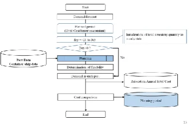
Setting of Target Period and Simulation Design

Figure 1. Simulation flowchart.

Verification with Actual Data

The following simulation verifies the proposed formulation model using actual data with Figure 2.

Figure 2. Requirements, storage, and handling costs for each port.

Figure 3 shows the results of a one-year simulation for the planning period. As the period considered in planning grows, it becomes possible to perform appropriate planning and reduce total costs. After 21 days, the fluctuation range of the total cost becomes smaller, and it becomes possible to formulate a container ship management plan.

Figure 3. Simulation results.

Conclusion

We proposed a formulation method for relocation of empty containers, and developed a simulation that can be reproduced and verified. We were able to verify the effectiveness of the proposed method using actual data.

References

[1] Song, Dong-Ping, and Jing-Xin Dong. “Effectiveness of an Empty Container Repositioning Policy with Flexible Destination Ports.” Transport Policy 18, no. 1 (January 2011): 92–101.

[3] Tran, Nguyen Khoi, and Hans-Dietrich Haasis. “Literature Survey of Network Optimization in Container Liner Shipping.” Flexible Services and Manufacturing Journal 27, no. 2–3 (June 19, 2013): 139–79.

[4] Drewry (2011), Container market—annual review and forecast. Drewry Shipping Consultants, London.

[5] Crinks, P. (2000) Container Usage Asset Management in the Global Container Logistics Chain,

International Asset Systems.

[6] Song, Dong-Ping, and Jing-Xin Dong. “Cargo Routing and Empty Container Repositioning in Multiple Shipping Service Routes.” Transportation Research Part B: Methodological 46, no. 10 (December 2012): 1556–75.

[7] Song, D., and Q. Zhang. “A Fluid Flow Model for Empty Container Repositioning Policy with a Single Port and Stochastic Demand.” SIAM Journal on Control and Optimization 48, no. 5 (January 1, 2010): 3623–42.

[8] Wong, Eugene Y. C., Allen Tai, and Mardjuki Raman (2015) “A Maritime Container Repositioning Yield-Based Optimization Model with Uncertain Upsurge Demand.” Transportation Research Part E: Logistics and Transportation Review 82.

[9] Zheng, Jianfeng, Zhuo Sun, and Ziyou Gao (2015) “Empty Container Exchange among Liner Carriers.” Transportation Research Part E: Logistics and Transportation Review 83.

[10] Furió, Salvador, Carlos Andrés, Belarmino Adenso-Díaz, and Sebastián Lozano (2013) “Optimization of Empty Container Movements Using Street-Turn: Application to Valencia Hinterland.” Computers & Industrial Engineering 66, no. 4.