Computational Analysis of the Menu of U S – Japan Trade Policies

(1)

I

NTERNATIONAL

P

OLICY

C

ENTER

Gerald R. Ford School of Public Policy

University of Michigan

IPC Working Paper Series Number 108

Computational Analysis of the Menu of U.S. – Japan Trade Policies

Drusilla K. Brown

Kozo Kiyota

Robert M. Stern

(2)

Drusilla K. Brown, Tufts University

Kozo Kiyota, Yokohama National University

Robert M. Stern, University of Michigan

Abstract

We have used the Michigan Computable General Equilibrium (CGE) Model of World Production and Trade to calculate the aggregate welfare and sectoral employment effects of the menu of U.S.-Japan trade policies. The menu of policies encompasses the various preferential U.S. and Japan bilateral and regional free trade agreements (FTAs) negotiated and in process, unilateral removal of existing trade barriers by the two countries, and global (multilateral) free trade. The U.S. preferential agreements include the FTAs approved by the U.S. Congress with Chile and Singapore in 2003, those signed with Central America, Australia, and Morocco and receiving Congressional approval in 2004, and prospective FTAs with the Southern African Customs Union (SACU), Thailand, and the Free Trade Area of the Americas (FTAA). The Japanese preferential agreements include the bilateral FTA with Singapore signed in 2002 and prospective FTAs with Chile, Indonesia, Korea, Malaysia, Mexico, Philippines, and Thailand. The welfare impacts of the FTAs on the United States and Japan are shown to be rather small in absolute and relative terms. The sectoral employment effects are also generally small in the United States and Japan, but vary across the individual sectors depending on the patterns of the bilateral liberalization. The welfare effects on the FTA partner countries are mostly positive though generally small, but there are some indications of potentially disruptive employment shifts in some partner countries. There are indications of trade diversion and detrimental welfare effects on nonmember countries for some of the FTAs analyzed. Data limitations precluded analysis of the welfare effects of the different FTA rules of origin and other discriminatory arrangements.

In comparison to the welfare gains from the U.S. and Japan bilateral FTAs, the gains from both unilateral trade liberalization by the United States, Japan, and the FTA partners, and from global (multilateral) free trade are shown to be rather substantial and more uniformly positive for all countries in the global trading system. The U.S. and Japan FTAs are based on "hub" and "spoke" arrangements. We show that the spokes emanate out in different and often overlapping directions, suggesting that the complex of bilateral FTAs may create distortions of the global trading system.

Keywords: Multilateral, Regional, and Bilateral Trade Liberalization; JEL: F10; F13; F15

October 8, 2010

Citation: Drusilla K. Brown, Kozo Kiyota, Robert M. Stern (2010), Chapter 11 Computational Analysis of the Menu of U.S.–Japan Trade Policies, in Professor Hamid Beladi, Professor E. Kwan Choi (ed.) New Developments in Computable General Equilibrium Analysis for Trade Policy

(3)

Drusilla K. Brown, Tufts University Kozo Kiyota, Yokohama National University**

Robert M. Stern, University of Michigan

I. Introduction

In this paper, we present a computational analysis of the economic effects of the menu of

U.S.-Japan trade policies. The menu encompasses the various U.S. and Japan bilateral and

regional free trade agreements (FTAs) that had been negotiated and the negotiations currently in

process in August 2004 when this paper was originally written, unilateral removal of existing

trade barriers by the United States, Japan, and their FTA partner countries, and global

(multilateral) free trade. The analysis is based on the Michigan Model of World Production and

Trade. The Michigan Model is a multi-country/multi-sector computable general equilibrium

(CGE) model of the global trading system that has been used for more than three decades to

analyze the economic effects of multilateral, regional, and bilateral trade negotiations and a

variety of other changes in trade and related policies.

In Section II following, we present a brief description of the main features and data of the

Michigan Model. The results of the computational analysis of the U.S. and Japan FTAs are

presented in Sections III and IV. In Section V, we consider the cross-country patterns of the

welfare effects of the various FTAs. In Section VI, we provide a broader perspective on the

FTAs that takes into account the effects of the unilateral and multilateral removal of trade barriers

by the United States and Japan, their FTA partner countries, and other countries/regions in the

global trading system. Section VII provides a summary and concluding remarks.

________________________

*This paper has been adapted from Brown, Kiyota, and Stern (2006). We wish to thank Masahiko Tsutsumi and participants in the March 2004 pre-conference meeting in Ann Arbor and the May 2004 Tokyo conference for helpful comments on earlier versions of the paper.

(4)

II. The Michigan Model of World Production and Trade

Overview of the Michigan Model

The version of the Michigan Model that we use in this paper covers 18 economic sectors,

including agriculture, manufactures, and services, in each of 22 countries/regions. The

distinguishing feature of the Michigan Model is that it incorporates some aspects of trade with

imperfect competition, including increasing returns to scale, monopolistic competition, and product

variety. Some details follow.1 A more complete description of the formal structure and equations

of the model can be found on line at www.Fordschool.umich.edu/rsie/model/.

Sectors and Market Structure

As mentioned, the version of the model used consists of 18 production sectors and 22

countries/regions (plus rest-of-world). The sectoral and country/region coverage are indicated in

the tables below. Agriculture is modeled as perfectly competitive with product differentiation by

country of origin, and all other sectors covering manufactures and services are modeled as

monopolistically competitive. Each monopolistically competitive firm produces a differentiated

product and sets price as a profit-maximizing mark-up of price over marginal cost. Free entry and

exit of firms then guarantees zero profits.

Expenditure

Consumers and producers are assumed to use a two-stage procedure to allocate expenditure

across differentiated products. In the first stage, expenditure is allocated across goods without

regard to the country of origin or producing firm. At this stage, the utility function is Cobb-Douglas,

and the production function requires intermediate inputs in fixed proportions. In the second stage,

expenditure on monopolistically competitive goods is allocated across the competing varieties

supplied by each firm from all countries. In the perfectly competitive agricultural sector, since

1

(5)

individual firm supply is indeterminate, expenditure is allocated over each country’s sector as a

whole, with imperfect substitution between products of different countries.

The aggregation function in the second stage is a Constant Elasticity of Substitution (CES)

function. Use of the CES function and product differentiation by firm imply that consumer welfare

is influenced both by any reduction in real prices brought about by trade liberalization, as well as

increased product variety. The elasticity of substitution among different varieties of a good is

assumed to be three, a value that is broadly consistent with available empirical estimates. The

parameter for the sensitivity of consumers to the number of product varieties is set at 0.5.2

Production

The production function is separated into two stages. In the first stage, intermediate inputs

and a primary composite of capital and labor are used in fixed proportion to output.3 In the second

stage, capital and labor are combined through a CES function to form the primary composite. In the

monopolistically competitive sectors, additional fixed inputs of capital and labor are required. It is

assumed that fixed capital and fixed labor are used in the same proportion as variable capital and

variable labor so that production functions are homothetic. The elasticities of substitution between

capital and labor vary across sectors and were derived from a literature search of empirical

estimates of sectoral supply elasticities. Economies of scale are determined endogenously in the

model.

Supply Prices

To determine equilibrium prices, perfectly competitive firms operate such that price is

equal to marginal cost, while monopolistically competitive firms maximize profits by setting price

as an optimal mark-up over marginal cost. The numbers of firms in sectors under monopolistic

2

If the variety parameter is greater than 0.5, it means that consumers value variety more. If the parameter is zero, consumers have no preference for variety. This is the same as the Armington assumption according to which consumers view products as distinguished by country of production. Sensitivity tests of

alternative parameter values are included in an appendix below. 3

(6)

competition are determined by the zero profits condition. The free entry condition in this context is

also the basic mechanism through which new product varieties are created (or eliminated). Each of

the new entrants arrives with a distinctly different product, expanding the array of goods available

to consumers.

Free entry and exit are also the means through which countries are able to realize the

specialization gains from trade. In this connection, it can be noted that in a model with nationally

differentiated products, which relies on the Armington assumption, production of a particular

variety of a good cannot move from one country to another. In such a model, there are gains from

exchange but no gains from specialization. However, in the Michigan Model with differentiated

products supplied by monopolistically competitive firms, production of a particular variety is

internationally mobile. A decline in the number of firms in one country paired with an expansion in

another essentially implies that production of one variety of a good is being relocated from the

country in which the number of firms is declining to the country in which the number of firms is

expanding. Thus, we have both an exchange gain and a specialization gain from international

trade.4

Capital and Labor Markets

Capital and labor are assumed to be perfectly mobile across sectors within each country.

Returns to capital and labor are determined so as to equate factor demand to an exogenous supply of

each factor. The aggregate supplies of capital and labor in each country are assumed to remain fixed

so as to abstract from macroeconomic considerations (e.g., the determination of investment), since

our microeconomic focus is on the inter-sectoral allocation of resources.

4

(7)

World Market and Trade Balance

The world market determines equilibrium prices such that all markets clear. Total demand

for each firm or sector’s product must equal total supply of that product. It is also assumed that

trade remains balanced for each country/region, that is, any initial trade imbalance remains constant

as trade barriers are changed. This is accomplished by permitting aggregate expenditure to adjust to

maintain a constant trade balance. Thus, we abstract away from the macroeconomic forces and

policies that are the main determinants of trade imbalances. Further, it should be noted that there

are no nominal rigidities in the model. As a consequence, there is no role for a real exchange rate

mechanism.

Trade Policies and Rent/Revenues

We have incorporated into the model the import tariff rates and export taxes/subsidies as

policy inputs that are applicable to the bilateral trade of the various countries/regions with respect

to one another. These have been computed using the "GTAP–5.4 Database" provided in

Dimaranan and McDougall (2002). This was the latest database available at the time of writing

in 2006. The export barriers have been estimated as export-tax equivalents. We assume that

revenues from both import tariffs and export taxes, as well as rents from NTBs on exports, are

redistributed to consumers in the tariff- or tax-levying country and are spent like any other

income.

Tariff liberalization can affect economic efficiency through three main channels. First, in

the context of standard trade theory, tariff reductions both reduce the cost of imports for consumers

and for producers purchasing traded intermediate inputs, thus producing an exchange gain. Second,

tariff removal leads firms to direct resources toward those sectors that have the greatest value on the

world market. That is, we have the standard specialization gain. Third, tariff reductions have a

pro-competitive effect on sellers. Increased price pressure from imported varieties force incumbent

(8)

average total cost (ATC) curve. The consequent lower ATC of production creates gains from the

realization of economies of scale.

Model Closure and Implementation

We assume in the model that aggregate expenditure varies endogenously to hold aggregate

employment constant. This closure is analogous to the Johansen closure rule (Deardorff and Stern,

1990, pp. 27-29). The Johansen closure rule consists of keeping the requirement of full employment

while dropping the consumption function. This means that consumption can be thought of as

adjusting endogenously to ensure full employment. However, in the present model, we do not

distinguish consumption from other sources of final demand. That is, we assume instead that total

expenditure adjusts to maintain full employment.

The model is solved using GEMPACK (Harrison and Pearson, 1996). When policy

changes are introduced into the model, the method of solution yields percentage changes in sectoral

employment and certain other variables of interest. Multiplying the percentage changes by the

absolute levels of the pertinent variables in the database yields the absolute changes, positive or

negative, which might result from the various liberalization scenarios.

Interpreting the Modeling Results

To help the reader interpret the modeling results, it is useful to review the features of the

model that serve to identify the various economic effects to be reflected in the different

applications of the model. Although the model includes the aforementioned features of imperfect

competition, it remains the case that markets respond to trade liberalization in much the same way

that they would with perfect competition. That is, when tariffs or other trade barriers are reduced

in a sector, domestic buyers (both final and intermediate) substitute toward imports and the

domestic competing industry contracts production while foreign exporters expand. Thus, in the

case of multilateral liberalization that reduces tariffs and other trade barriers simultaneously in

(9)

contracting depending primarily on whether their protection is reduced more or less than in other

sectors and countries.

Worldwide, these changes cause increased international demand for all sectors. World

prices increase most for those sectors where trade barriers fall the most.5 This in turn causes

changes in countries’ terms of trade that can be positive or negative. Those countries that are net

exporters of goods with the greatest degree of liberalization will experience increases in their

terms of trade, as the world prices of their exports rise relative to their imports. The reverse

occurs for net exporters in industries where liberalization is slight – perhaps because it may

already have taken place in previous trade rounds.

The effects on the welfare of countries arise from a mixture of these terms-of-trade

effects, together with the standard efficiency gains from trade and also from additional benefits

due to the realization of economies of scale. Thus, we expect on average that the world will gain

from multilateral liberalization, as resources are reallocated to those sectors in each country

where there is a comparative advantage. In the absence of terms-of-trade effects, these efficiency

gains should raise national welfare measured by the equivalent variation for every country,6

although some factor owners within a country may lose, as will be noted below. However, it is

possible for a particular country whose net imports are concentrated in sectors with the greatest

liberalization to lose overall, if the worsening of its terms of trade swamps these efficiency gains.

On the other hand, although trade with imperfect competition is perhaps best known for

introducing reasons why countries may lose from trade, actually its greatest contribution is to

expand the list of reasons for gains from trade. Thus, in the Michigan Model, trade liberalization

permits all countries to expand their export sectors at the same time that all sectors compete more

5

The price of agricultural products supplied by the rest of the world is taken as the numeraire in the model, and there is a rest-of-world against which all other prices can rise.

6

(10)

closely with a larger number of competing varieties from abroad. As a result, countries as a

whole gain from lower costs due to increasing returns to scale, lower monopoly distortions due to

greater competition, and reduced costs and/or increased utility due to greater product variety. All

of these effects make it more likely that countries will gain from liberalization in ways that are

shared across the entire population.7

The various effects just described in the context of multilateral trade liberalization will

also take place when there is unilateral trade liberalization, although these effects will depend on

the magnitudes of the liberalization in relation to the patterns of trade and the price and output

responses involved between the liberalizing country and its trading partners. Similarly, many of

the effects described will take place with the formation of bilateral or regional FTAs. But in these

cases, there may be trade creation and positive effects on the economic welfare of FTA-member

countries together with trade diversion and negative effects on the economic welfare of

non-member countries. The net effects on economic welfare for individual countries and globally will

thus depend on the economic circumstances and policy changes implemented.8

In the real world, all of the various effects occur over time, some of them more quickly

than others. However, the Michigan Model is static in the sense that it is based upon a single set

of equilibrium conditions rather than relationships that vary over time.9 The model results

7

In perfectly competitive trade models such as the Heckscher-Ohlin Model, one expects countries as a whole to gain from trade, but the owners of one factor – the "scarce factor" – to lose through the mechanism first explored by Stolper and Samuelson (1941). The additional sources of gain from trade due to increasing returns to scale, competition, and product variety, however, are shared across factors, and we routinely find in our CGE modeling that both labor and capital gain from multilateral trade liberalization. 8

It may be noted that, in a model of perfect competition, bilateral trade liberalization should have the effect of contracting trade with the excluded countries, thereby improving the terms of trade for the FTA members vis-à-vis the rest of world. But in a model with scale economies, the pro-competitive effect of trade liberalization can generate a cut in price and increase in supply to excluded countries. The terms of trade of FTA members may therefore deteriorate in this event.

It should also be mentioned that rules of origin may offset some of the potential welfare benefits of FTAs insofar as they may lead to higher input costs and consequent reduction of FTA preference margins. In this connection, see Krishna (2004).

9

(11)

therefore refer to a time horizon that depends on the assumptions made about which variables do

and do not adjust to changing market conditions, and on the short- or long-run nature of these

adjustments. Because the supply and demand elasticities used in the model reflect relatively

long-run adjustments and it is assumed that markets for both labor and capital clear within

countries,10 the modeling results are appropriate for a relatively long time horizon of several

years – perhaps two or three at a minimum. On the other hand, the model does not allow for the

very long-run adjustments that could occur through capital accumulation, population growth, and

technological change. The modeling results should therefore be interpreted as being

superimposed upon longer-run growth paths of the economies involved. To the extent that these

growth paths themselves may be influenced by trade liberalization, therefore, the model does not

capture such effects.

Benchmark Data

Needless to say, the data needs of this model are immense. Apart from numerous share

parameters, the model requires various types of elasticity measures. Like other CGE models,

most of our data come from published sources.

As mentioned above, the main data source used in the model is "The GTAP-5.4 Database"

of the Purdue University Center for Global Trade Analysis Project (Dimaranan and McDougall,

2002). The reference year for this GTAP database is 1997. From this source, we have extracted

the following data, aggregated to our sectors and countries/regions:11

net tax and tariff revenues to be redistributed to consumers, when tariffs are reduced with trade liberalization, the model implicitly imposes a non-distorting tax to recoup the loss in tariff revenues.

10

The analysis in the model assumes throughout that the aggregate, economy-wide, level of employment is held constant in each country. The effects of trade liberalization are therefore not permitted to change any country's overall rates of employment or unemployment. This assumption is made because overall employment is determined by macroeconomic forces and policies that are not contained in the model and would not themselves be included in a negotiated trade agreement. The focus instead is on the composition of employment across sectors as determined by the microeconomic interactions of supply and demand resulting from the liberalization of trade.

11

(12)

• Bilateral trade flows among 22 countries/regions, decomposed into 18 sectors. Trade with the rest-of-world (ROW) is included to close the model.

• Input-output tables for the 22 countries/regions, excluding ROW

• Components of final demand along with sectoral contributions for the 22 countries/regions, excluding ROW

• Gross value of output and value added at the sectoral level for the 22 countries/regions, excluding ROW

• Bilateral import tariffs by sector among the 22 countries/regions

• Elasticity of substitution between capital and labor by sector

• Bilateral export-tax equivalents among the 22 countries/regions, decomposed into 18 sectors

The monopolistically competitive market structure in the nonagricultural sectors of the

model imposes an additional data requirement of the numbers of firms at the sectoral level, and

there is need also for estimates of sectoral employment.12 The employment data, which have

been adapted from a variety of published sources, will be noted in tables below.

The GTAP-5.4 1997 database has been projected to the year 2005, which is when the

Uruguay Round liberalization will have been fully implemented. In this connection, we

extrapolated the labor availability in different countries/regions by an average weighted

population growth rate of 1.2 percent per annum. All other major variables have been projected,

using an average weighted growth rate of GDP of 2.5 percent.13 The 2005 data have been

adjusted to take into account two major developments that have occurred in the global trading

system since the mid-1990s. These include: (1) implementation of the Uruguay Round

negotiations that were completed in 1993-94 and were to be phased in over the following decade;

12

Notes on the construction of the data on the number of firms and for employment are available from the authors on request.

13

(13)

and (2) the accession of Mainland China and Taiwan to the WTO in 2001.14 We have made

allowance for the foregoing developments by readjusting the 2005 scaled-up database for

benchmarking purposes to obtain an approximate picture of what the world may be expected to

look like in 2005. In the computational scenarios to be presented below, we use these re-adjusted

data as the starting point to carry out our liberalization scenarios for the U.S. bilateral FTAs and

for the accompanying unilateral and global free trade scenarios.

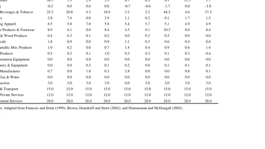
The GTAP 5.4 (1997) base data for tariffs and the estimated tariff equivalents of services

barriers are broken down by sector on a global basis and bilaterally for existing and prospective

FTA partners of the United States and Japan in Tables 1-2. The post-Uruguay Round tariff rates

on agriculture, mining, and manufactures are applied rates and are calculated in GTAP by

dividing tariff revenues by the value of imports by sector.

The services barriers are based on financial data on average gross (price-cost) margins

constructed initially by Hoekman (2000) and adapted for modeling purposes in Brown, Deardorff,

and Stern (2002). The gross operating margins are calculated as the differences between total

revenues and total operating costs. Some of these differences are presumably attributable to fixed

costs. Given that the gross operating margins vary across countries, a portion of the margin can

also be attributed to barriers to FDI. For this purpose, a benchmark is set for each sector in

relation to the country with the smallest gross operating margin, on the assumption that

operations in the benchmark country can be considered to be freely open to foreign firms. The

excess in any other country above this lowest benchmark is then taken to be due to barriers to

establishment by foreign firms.

14

(14)

That is, the barrier is modeled as the cost-increase attributable to an increase in fixed cost

borne by multinational corporations attempting to establish an enterprise locally in a host country.

This abstracts from the possibility that fixed costs may differ among firms because of variations

in market size, distance from headquarters, and other factors. It is further assumed that this cost

increase can be interpreted as an ad valorem equivalent tariff on services transactions generally.

It can be seen in Tables 1 and 2 that the constructed services barriers are considerably higher than

the import barriers on manufactures. While possibly subject to overstatement, it is generally

acknowledged that many services sectors are highly regulated and thus restrain international

services transactions.

For the United States, the highest import tariffs for manufactures are recorded for textiles,

wearing apparel, and leather products & footwear, both globally and bilaterally. For Japan, the

highest import tariffs are noted in agriculture, food, beverages & tobacco, textiles, wearing

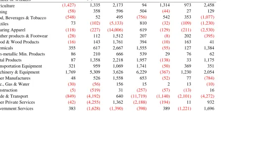
apparel, and leather & leather products. The values and shares of U.S. and Japanese exports and

imports are broken down by sector according to origin and destination in Tables 3-6 on a global

basis as well as for FTA partners. Employment by sector is indicated for the United States and

for Japan and their FTA partners in Table 7.

III. Computational Analysis of U.S. Free Trade Agreements

As already noted, both the United States and Japan had signed or were in the process of

negotiating bilateral FTAs in 2006, at the time of writing. For the United States, these include the

agreements with Chile and Singapore approved by the U.S. Congress in 2003, agreements with

Central America and the Dominican Republic (CAFTA), Australia, and Morocco to be submitted

for Congressional approval in 2004, and ongoing negotiations with the Southern African Customs

Union (SACU), Thailand, and the Free Trade Area of the Americas (FTAA).15 The Japanese

15

(15)

bilateral FTAs will be analyzed below and include the agreement with Singapore signed in 2002

and subsequent and prospective agreements with Chile, Korea, Malaysia, Mexico, Philippines,

and Thailand.

As we note in Brown, Kiyota, and Stern (2005a,b,2007,2008), the United States has a

myriad of objectives in pursuing FTAs, including increased market access and shaping the

regulatory and political environment in FTA partner countries to conform to U.S. principles and

institutions. By the same token, the FTA partners are attracted by the preferential margins for

U.S. market access and opportunities to improve their economic efficiency and to design and

implement more effective domestic institutions and policies. Similarly, Japan and its FTA

partners are motivated by many of these objectives.

The U.S. FTAs to be analyzed are denoted as follows:

USCHFTA U.S.-Chile FTA

USSGFTA U.S.-Singapore FTA

USCAFTA U.S.-Central America FTA

USAUSFTA U.S.-Australia FTA

USMORFTA U.S.-Morocco FTA

USSACUFTA U.S.-Southern African Customs Union FTA USTHFTA U.S.-Thailand FTA

FTAA Free Trade Area of the Americas

Our reference point is the Uruguay Round 2005 database together with the

post-Uruguay Round tariff rates on agricultural products and manufactures and the specially

constructed measures of services barriers described above. Four scenarios have been carried out

for each FTA: (A) removal of agricultural tariffs16; (M) removal of manufactures tariffs; (S)

removal of services barriers; and (C) combined removal of agricultural and manufactures tariffs

and services barriers. Because of space constraints, we report only the results of the combined

with Bahrain in 2004. An FTA with Peru was approved in 2009. Negotiations have been ongoing with Colombia, Korea, and Panama and are yet to be submitted for Congressional approval. See the USTR website for more information.

16

(16)

removal of agricultural and manufactures tariffs and services barriers, denoted by USCHFTA-C,

etc. The results for the separate removal of the agricultural, manufactures, and services barriers

and for the sectoral effects on exports, imports, and gross output are available on request.

We should emphasize that our computational analysis does not take into account other

features of the various FTAs, which do not lend themselves readily to quantification. These other

features cover E-commerce, intellectual property, labor and environmental standards, investment,

government procurement, trade remedies, dispute settlement, and the development of new

institutional and cooperative measures. By the same token, because of data constraints, we have

not made allowance for rules of origin and special preferences that may be negotiated as part of

each FTA and that could be designed for protectionist reasons to limit trade.

USCHFTA-C: U.S.-Chile Free Trade Agreement – The U.S.-Chile FTA was approved

by the U.S. Congress in 2003. The estimated global welfare effects are indicated in Table 8.

Global welfare increases by $7.9 billion, with U.S. welfare increasing by $6.9 billion (0.1% of

GNP) and Chile’s welfare by $1.2 billion (1.3% of GNP).17 The sectoral results for the United

States are shown in Table 9 and indicate relatively small employment declines in U.S. agriculture,

food, beverages & tobacco, wearing apparel, and leather products & footwear, and employment

increases in the other sectors. The sectoral employment effects for Chile are indicated in Table

10 and show employment increases in agriculture, mining, food, beverages & tobacco, leather &

leather products, metal products, and trade and transport services, and employment declines in

several manufacturing sectors and other services. These employment changes for Chile suggest

the extent of labor market adjustments that may occur as a result of the FTA.

USSGFTA-C: U.S.-Singapore Free Trade Agreement – The welfare effects of a

U.S.-Singapore FTA, which was approved by the U.S. Congress in 2003, noted in Table 8, indicate an

increase in global welfare of $22.5 billion, with U.S. welfare rising by $15.8 billion (0.2% of

17

(17)

GNP) and Singapore’s welfare by $2.5 billion (2.6% of GNP). In Table 9, the sectoral

employment effects for the United States are relatively small, whereas in Table 10, for Singapore,

there are relatively large sectoral employment increases in textiles, wearing apparel, and services,

and declines in most other sectors. These sectoral changes suggest sizable employment

adjustments for Singapore that may occur in the FTA with the United States.

USCAFTA-C: U.S.-Central America Free Trade Agreement – The U.S.-CAFTA was

signed in December 2003 and was subsequently approved by the U.S. Congress. The estimated

global welfare effects are shown in Table 8. Global welfare rises by $15.7 billion, U.S. welfare

by $17.3 billion (0.2% of GNP) and the welfare of the aggregate of Central American and the

Caribbean (CAC) by $5.3 (4.4% of GNP).18,19 It can also be seen that the CAFTA is apparently

trade diverting for most of the non-member countries/regions shown. The sectoral employment

effects for the United States, noted in Table 9, indicate that. the employment declines are

concentrated in textiles and wearing apparel and are comparatively small as a percent of

employment in these sectors, -0.6% and -1.8%, respectively. The sectoral employment changes

18

The GTAP 5.4 data refer to a CAC aggregate and do not provide separate data for the five Central American countries and the Dominican Republic that comprise the CAFTA. It is noted in Brown, Kiyota, and Stern (2005b) that the CAFTA countries account for a substantial proportion of CAC trade so that using CAC data may be a reasonable approximation for modeling purposes.

19

Andriamananjara and Tsigas (2003) use the standard GTAP model to analyze the welfare effects of bilateral U.S. FTAs with 65 countries/regions. This version of the GTAP model assumes constant returns to scale, perfect competition, and product differentiation by country of origin (the so-called Armington assumption). The Armington assumption implies that countries have monopoly power in their trading relationships, and that trade liberalization may thus have sizable terms-of-trade effects, depending on the structure and pattern of trade. There is reason to believe accordingly that welfare changes in this version of the GTAP model may reflect strong terms-of-trade effects. This is evident in the results of a U.S.-CAC FTA, which is estimated to increase U.S. economic welfare by $1.6 billion (.02% of GDP) and CAC welfare by $2.2 billion (2.4% of GDP). The decomposition of the results by the authors in their Appendix Table indicates that a substantial proportion of these welfare changes is due to changes in terms of trade. DeRosa and Gilbert (2004) also use the standard GTAP model to analyze U.S. bilateral FTAs with 13 prospective partner countries, and their results similarly suggest the predominance of terms of trade effects. In contrast, in the Michigan Model, manufactures and services products are differentiated by firm, so that countries have much less leverage over their terms of trade.

(18)

for the CAC are shown in Table 10. The increases are quite large in textiles, wearing apparel,

and leather products & footwear, and there are employment declines in all of the other sectors, as

the expansion of the relatively labor-intensive industries attracts workers from the rest of the

economy. These results thus suggest that the CAFTA may result in significant worker

displacement in the process of adjustment brought about by elimination of the import barriers.

USAUSFTA-C: U.S.-Australia FTA – The U.S.-Australia FTA was signed in February

2004 and was later approved by the U.S. Congress. It can be seen in Table 8 that global welfare

rises by $23.1 billion, U.S. welfare by $19.4 billion (0.2% of GNP), and Australian welfare by 5.4

billion (1.1% of GNP). There are many instances of trade diversion for non-partner countries. The

sectoral effects for the United States in Table 9 and for Australia in Table 10 indicate that the

U.S.-Australia FTA will have fairly small effects on the sectoral employment in the two

countries.

USMORFTA-C: U.S.-Morocco FTA – As noted in Tables 3-4 above, U.S. trade in

goods and services with Morocco is rather small. By far the largest proportions of Morocco’s

trade are with the EU and EFTA. The global welfare increase from the U.S.-Morocco FTA

indicated in Table 8 is $7.5 billion, $6.0 billion (0.1% of GNP) for the United States, and $0.9

billion (2.0% of GNP) for Morocco.20 The U.S. sectoral employment changes noted in Table 9

are negligible. For Morocco, in Table 10, the largest employment increases are in trade &

transport, textiles, and wearing apparel, and the largest declines in agriculture, food, beverages &

tobacco, and government services. The welfare and employment effects of the U.S.-Morocco

FTA are thus seen to be fairly small.

USSACUFTA-C: U.S.-Southern African Customs Union – The effects of a

U.S.-SACU FTA are indicated in Table 8 and indicate an increase of $11.8 billion in global welfare,

20

(19)

$9.6 billion (0.1% of GNP) for the United States, and $2.2 billion (1.2% of GNP) for the SACU

members combined. In Table 9, there are indications of negligible sectoral employment impacts

for the United States. In Table 10, the employment increases for SACU are concentrated in

textiles and wearing apparel and are negative across the remaining sectors as labor is attracted

towards the labor-intensive sectors.

US-THFTA-C: U.S.-Thailand FTA – In Table 8, the global welfare increase for the

U.S.-Thailand FTA is $21.9 billion, $17.1 billion (0.2% of GNP) for the United States, and $5.6

billion (2.8% of GNP) for Thailand. There is evidence of pervasive trade diversion. The sectoral

employment changes for the United States noted in Table 9 are negligible. For Thailand, in Table

10, the largest employment increases are concentrated in food, beverages & tobacco, textiles,

wearing apparel, leather & leather products, other manufactures, and trade & transport, and there

are employment declines especially in agriculture, mining, several capital-intensive manufactures,

construction, other private services, and government services.

FTAA-C: Free Trade Area of the Americas – Discussions have been ongoing for

several years to create a Free Trade Area for the Americas (FTAA).21 Since the country detail in

our model does not include the individual members of the FTAA, we have chosen to approximate

it by combining the United States, Canada, Mexico, and Chile with an aggregate of Central

American and Caribbean (CAC) and an aggregate of other South American nations. The welfare

effects of the FTAA are indicated in column Table 8 and amount to $109.5 billion globally, $67.6

billion (0.7% of GNP) for the United States, $5.8 billion (0.7% of GNP) for Canada, $3.4 billion

(3.6% of GNP) for Mexico, $3.4 billion (3.6% of GNP) for Chile, $7.8 billion (6.5% of GNP) for

the CAC, and $27.6 billion (1.5% of GNP) for the aggregate of other South American countries.

There is some evidence of trade diversion, in particular for Japan and the EU/EFTA. The sectoral

employment effects for the United States, indicated in Table 11, show relatively small

21

(20)

employment declines in agriculture, mining, food, beverages & tobacco, and other private and

government services, and increases in all other sectors. In Table 11, the sectoral employment

effects for Canada are also small, whereas the employment increases for Mexico, Chile, the CAC,

and other South America are noteworthy. This suggests that the developing countries covered in

the FTAA would experience more employment adjustments than the United States and Canada.

IV. Computational Analysis of Japan’s Free Trade Agreements

In this section, we consider the welfare and sectoral employment effects of the

Japan-Singapore FTA that was concluded in 2002 and the FTAs in process with Chile, Indonesia,

Korea, Malaysia, Mexico, Philippines, and Thailand.22 These are designated as follows:

JSGFTA Japan-Singapore FTA

JCHFTA Japan-Chile FTA

JINDFTA Japan-Indonesia FTA

JKFTA Japan-Korea FTA

JMAFTA Japan-Malaysia FTA

JMXFTA Japan-Mexico FTA

JPHFTA Japan-Philippines FTA

JTHFTA Japan-Thailand FTA

As was the case for the U.S. FTAs analyzed in the previous section, we have undertaken

separate computations for (A) removal of agricultural tariffs; (M) removal of manufactures

tariffs; (S) removal of services barriers; and (C) combined removal of agricultural and

manufactures tariffs and services barriers. In what follows, we report only the results of the

combined removal of agricultural and manufactures tariffs and services barriers, denoted by

JSGFTA-C, etc. The results for the separate removal of the agricultural, manufactures, and

services barriers are available on request.

22

(21)

JSGFTA-C: Japan-Singapore Free Trade Agreement – As shown in Table 12, the

combined removal of bilateral tariffs on agricultural products and manufactures and services

barriers would increase global economic welfare by $6.7 billion. Japan’s welfare rises by $5.0

billion (0.1% of GNP) and Singapore by $0.6 billion (0.7% of GNP). A JSGFTA appears to be

trade diverting to a small extent. The other industrialized countries besides Japan show increases

in welfare.23 The sectoral results, which are shown Table 13, indicate negligible shifts in Japan’s

employment. For Singapore, as indicated in Table 14, there are employment increases especially

in wearing apparel, leather & leather products, and trade & transport, and declines in many other

manufacturing sectors and other private services. A Japan-Singapore FTA thus appears to have

relatively small effects on Japan’s welfare and results in sectoral employment shifts in Singapore

away from capital-intensive towards relatively more labor-intensive sectors.

JCHFTA-C: Japan-Chile Free Trade Agreement – In Table 12, a JCHFTA indicates

increases in global welfare of $3.5 billion. Japan’s welfare rises by $2.8 billion (0.1% of GNP),

and Chile’s welfare rises by $0.9 billion (1.0% of GNP). There are negative welfare effects for

the United States, Canada, and several developing countries. The sectoral results for Japan, in

Table 13, indicate negligible sectoral shifts. For Chile, as indicated in Table 14, there are

employment increases in agriculture and food, beverages & tobacco and declines in mining and

all of the manufactures and services sectors as resources are shifted away from these sectors.

JINDFTA-C: Japan-Indonesia Free Trade Agreement – As indicated in Table 12, a

JINDFTA increases global welfare by $11.1 billion, Japan’s welfare by $18.7 billion (0.2% of

GNP), and Indonesia’s welfare by $1.7 billion (0.7% of GNP). There are indications of trade

diversion and negative welfare effects for most of the non-member countries/regions. The

23

(22)

sectoral results for Japan in Table 13 show small negative employment effects on Japanese

agriculture and labor-intensive manufactures and positive effects on most other sectors. For

Indonesia, the sectoral employment effects mirror those in Japan, with employment expansion in

Indonesian agriculture, food, beverages & tobacco, and labor-intensive manufactures and

employment declines in all other sectors.

JKFTA-C: Japan-Korea Free Trade Agreement – In Table 12, a JKFTA increases

global welfare by $19.7 billion, Japan’s welfare by $18.7 billion (0.4% of GNP), and Korea’s

welfare increases by $2.2 billion (0.4% of GNP). There is some evidence of trade diversion for

the United States, EU/EFTA, and for some developing countries. The sectoral results, shown in

Table 13, indicate relatively small employment declines in Japan in agriculture and

labor-intensive manufactures, and increases in employment in durable manufactures and services. For

Korea, as shown in Table 14, employment falls in many capital-intensive manufactures sectors

and in services and rises in Korea’s agriculture and labor-intensive manufactures.24

JMAFTA-C: Japan-Malaysia Free Trade Agreement – Global economic welfare is

shown in Table 12 to increase by $10.1 billion, Japan’s welfare by $10.5 billion (0.2% of GNP),

and Malaysia’s welfare by $0.3 billion (0.2% of GNP). In Table 13, sectoral employment

declines in Japan’s agriculture, food, beverages & tobacco, labor-intensive sectors, machinery &

equipment, and other manufactures, and there are employment increases in the other

manufactures sectors and construction, other private services, and government services. For

Malaysia, in Table 14, the employment increases are concentrated in agriculture, food, beverages

& tobacco, wearing apparel, wood & wood products, and trade & transport, and there are declines

in capital-intensive manufactures and services except for trade & transport.

24

(23)

JMXFTA-C: Japan-Mexico Free Trade Agreement – As indicated in Table 12, a

JMXFTA increases global welfare by $10.6 billion. Japan’s welfare increases by $8.2 billion

(0.2% of GNP) and Mexico’s welfare by $3.4 billion (0.7% of GNP). There are indications that a

JMXFTA would be trade diverting for the United States, Canada, EU/EFTA , and several

developing countries. The sectoral results for Japan, shown in Table 13, indicate relatively small

employment declines in agriculture, food, beverages & tobacco, and labor-intensive manufactures

and increases especially in durable manufactures. For Mexico, in Table 14, the sectoral results

show relatively small employment increases in agriculture, food, beverages & tobacco, and trade

& transport and declines across the manufactures sectors and services.

JPHFTA-C: Japan-Philippines FTA – In Table 12, global welfare increases by $3.0

billion, Japan’s welfare by $2.2 billion (0.1% of GNP), and the Philippines welfare by $0.5

billion (0.6% of GNP). The sectoral employment results for Japan, noted in Table 13, indicate

declines in agriculture and food, beverages & tobacco, and labor-intensive manufactures and

increases in the other manufactures sectors and services. For the Philippines, in Table 14, the

employment shifts mirror those in Japan, with increases concentrated in agriculture, food,

beverages & tobacco and labor-intensive manufactures and declines across other manufactures

and services.

JTHFTA-C: Japan-Thailand FTA – In Table 12, a Japan-Thailand FTA increases

global welfare by $13.5 billion and Japan’s welfare by $19.5 billion (0.4% of GNP), and reduces

Thailand’s welfare by $0.5 billion (-0.3% of GNP). There are indications of trade diversion

across most of the other countries/regions indicated. There are sectoral employment declines in

Japan, noted in Table 13, in agriculture, food, beverages & tobacco, and labor-intensive sectors

and employment increases in capital-intensive manufactures and services. For Thailand, in Table

14, the employment increases are concentrated in agriculture and food, beverages & tobacco and

employment declines across the manufactures and services sectors. The reduction in Thailand’s

(24)

increasing returns to scale, to the agricultural sector, which is modeled with constant returns to

scale.

V. Hub and Spoke Effects of the U.S. and Japan FTAs

In the discussion of the U.S. and Japan bilateral FTAs in the preceding sections, it was

noted that there were indications of negative welfare effects for a number of non-member

countries/regions. It is well known theoretically that preferential trading arrangements may result

in both trade creation, which is welfare enhancing, and trade diversion, which will reduce welfare

as trade is shifted from lower to higher cost sources of supply. But there is another consideration,

which is that bilateral FTAs are based on the "hub-and-spoke" arrangement, with the United

States or Japan representing the hub and with separate spokes connecting the bilateral FTA

partners to the hub. In negotiating these bilateral FTAs, no account is taken of the effects that

they may have on non-members, even though there may be a bilateral FTA with one or more of

the non-members. As more and more bilateral FTAs are negotiated, the spokes of the FTAs may

thus emanate out in many different and overlapping directions, with resulting distortions of global

trade patterns. That is, this combination of varying preferences among different and overlapping

FTAs may lead to greatly increased transactions costs for firms and the undermining of the

most-favored-nation (MFN) principle of non-discrimination that is at the heart of the multilateral

trading system. These effects of the proliferation of FTAs are what Bhagwati and Panagariya

(1996) refer to as "spaghetti-bowl" effects.

An indication of the trade diversion associated with the U.S. and Japan FTAs and the

overlapping of the spokes involved is shown in the top half of Table 15, which has shaded cells

indicating cases of positive welfare effects and white cells indicating cases of negative welfare

effects. Altogether, 16 FTAs are shown, although there is some double counting insofar as the

U.S.-CAC and U.S.-Chile bilateral FTAs are encompassed in the FTAA. In any event, it seems

(25)

while partner-FTA countries may gain directly from their FTAs, as indicated by "X" in the table,

they may be adversely affected by other FTAs that have been negotiated.

The global results of the bilateral FTAs in Tables 8 and 12 above for the United States

and Japan suggest that the negative welfare effects on non-members may be rather small in both

absolute terms and as a percent of GNP. But, as mentioned in our earlier discussion, because of

data limitations, our results do not reflect the potential welfare declines due to rules of origin and

other discriminatory arrangements built into the bilateral FTAs. On the other hand, we do not

allow for increased inflows of foreign direct investment into the partner countries or the effects of

improvements in productivity and increased capital formation. Unfortunately, we are not in a

position to assess these potential benefits. But it seems clear from our computational results that

the welfare increases from the FTA removal of trade barriers are fairly small on the whole.

Pending further analysis, we therefore conclude that there is reason to be concerned about the

trade diversion and overlapping spoke effects of bilateral FTAs.

VI. Welfare Effects of Unilateral Free Trade and Global Free Trade

In this section, we ask how the welfare of the United States, Japan, their FTA partners,

and other countries/regions in the global trading system would be affected if it were feasible to

adopt unilateral free trade or global free trade on a non-discriminatory (MFN) basis. as compared

to the adoption of discriminatory bilateral FTAs. The results are indicated in Table 16. Unilateral

free trade adopted by the United States would increase U.S. welfare by $320.2 billion (3.2% of

GNP), which is about three times greater than the U.S. welfare gains from the bilateral FTAs

combined. If there were global (multilateral) free trade, U.S. welfare would be increased by

$401.8 billion (5.4% of GNP). Japan’s welfare would increase with unilateral free trade by

$200.3 billion (3.7% of GNP) and with global free trade by $542.5 billion (7.4% of GNP), as

compared to the $66.9 billion to be gained from Japan’s bilateral FTAs combined. There are also

(26)

unilateral free trade by the United States and Japan as compared to the partner-country gains from

their bilateral FTAs. Furthermore, the FTA partner countries would generally gain even more if

they adopted unilateral free trade and especially if there were global free trade.25

VII. Summary and Conclusions

In this paper, we have used the Michigan Model of World Production and Trade to

calculate the aggregate welfare and sectoral employment effects of the menu of U.S.-Japan trade

policies. The menu of policies encompasses the various preferential U.S. and Japan bilateral and

regional FTAs negotiated and in process, unilateral removal of existing trade barriers by the

United States, Japan, and the FTA partner countries, and global (multilateral) free trade. The

welfare impacts of the FTAs on the United States and Japan have been shown to be rather small

in absolute and relative terms. The sectoral employment effects are also generally small for both

countries, but vary across the individual sectors depending on the patterns of bilateral

liberalization.

The welfare effects on the FTA partner countries are shown to be mostly positive though

generally small, but there are some indications of potentially disruptive employment shifts in

some partner countries. The results further suggest that there would be trade diversion and

detrimental welfare effects in some non-member countries/regions. It also appears that, while

25

In commenting on an earlier version of our paper, Juan Carlos Hallak asked why there are larger absolute welfare gains and smaller percent changes in welfare for the large countries as compared to the small countries in our computational results. In this connection, the expectation is that, under conditions of perfect competition, a small country may appropriate a large share of the absolute gains from trade liberalization because the prices of the small country will tend to move towards the prices in the large country. Since large price changes give rise to large gains from trade, the small country may be expected therefore to realize greater gains from liberalization than the large country.

(27)

FTA partners may gain from the bilateral FTAs, they may be adversely affected because of

overlapping "hub-and-spoke" arrangements due to other discriminatory FTAs that have been

negotiated.

The welfare gains from both unilateral trade liberalization by the United States and Japan

and from global (multilateral) trade liberalization are shown to be rather substantial and more

uniformly positive for all countries/regions in the global trading system as compared to the

welfare gains from the bilateral FTAs analyzed.26 The issue then is whether and when the WTO

member countries will be able to overcome their divisiveness and indecisions and put the

multilateral negotiations back on track. The menu choice appears to be clear.

26

(28)

Appendix

Sensitivity Analysis

This appendix reports on sensitivity analysis of the Michigan Model. There are three key elasticities/parameters in the Model: the elasticity of substitution among varieties, which is exogenously set at three; the parameter that measures the sensitivity that consumers have to the number of varieties, which is set at 0.5; and the elasticities of supply that are taken from the literature.

The variety parameter can take on values between zero and one. The larger it is, it means that consumers value variety more. If the parameter is set at zero, consumers have no preference for variety. This would correspond to the Armington assumption, according to which consumers view products depending on their place of production..

To analyze the sensitivity of our model results, we have experimented with different values of the elasticity of substitution among varieties and the consumer sensitivity to the number of varieties. The following tests were conducted: (1) increase the elasticity of substitution among varieties by 10 percent, holding other parameters constant; (2) decrease the elasticity of

substitution by 10 percent, holding other parameters constant; (3) increase the consumption varieties parameter by 10 percent, holding other parameters constant; and (4) decrease the consumption varieties by 10 percent, holding other parameters constant.

The results, which are available on request, are not very sensitive to the alternative parameters of the consumption varieties. That is, a 10 percent increase (decrease) in these parameters yields only 2 percent larger (smaller) welfare effects compared to the baseline model. The sensitivity to the changes in the elasticity of substitution is large compared with the results of differences in the variety parameters. For some countries, the differences are greater than 10 percent

(29)

(Percent)

Global Singapore Australia Morocco SACU Thailand FTAA

Canada CAC Chile Mexico South

America

Agriculture 2.7 0.1 4.0 0.1 1.3 0.3 0.0 1.0 0.8 0.0 3.2

Mining 0.2 0.0 0.3 0.0 0.1 0.0 0.0 0.3 0.1 0.0 0.1

Food, Beverages & Tobacco 3.5 1.2 3.4 2.8 2.8 1.4 0.0 3.0 1.3 0.0 1.8

Textiles 5.7 9.3 6.5 7.1 6.3 8.7 0.0 6.8 14.0 0.0 7.7

Wearing Apparel 11.0 15.5 9.7 10.5 12.4 14.2 0.0 11.6 11.5 0.0 13.6

Leather Products &

Footwear 7.2 5.6 4.1 3.6 2.3 7.7 0.0 4.6 7.7 0.0 6.3

Wood & Wood Products 0.3 0.4 0.8 0.7 0.3 0.2 0.0 0.5 0.2 0.0 0.4

Chemicals 1.9 3.2 1.0 1.0 0.7 1.8 0.0 0.8 0.0 0.0 0.9

Non-metallic Min. Products 3.2 4.0 2.9 0.9 0.0 2.8 0.0 3.8 0.6 0.0 2.3

Metal Products 1.4 2.3 0.2 1.4 0.6 0.9 0.0 0.5 0.5 0.0 0.6

Transportation Equipment 1.2 1.0 1.5 0.3 1.7 0.1 0.0 1.3 1.4 0.0 0.2

Machinery & Equipment 1.0 0.8 1.6 0.0 0.1 0.1 0.0 0.3 0.2 0.0 0.4

Other Manufactures 1.3 1.3 0.9 0.0 0.4 0.4 0.0 2.2 0.1 0.0 1.5

Elec., Gas & Water 0.0 0.0 0.0 0.0 0.0 0.0 0.0 0.0 0.0 0.0 0.0

Construction 9.0 9.0 9.0 9.0 9.0 9.0 0.0 9.0 9.0 0.0 9.0

Trade & Transport 27.0 27.0 27.0 27.0 27.0 27.0 0.0 27.0 27.0 0.0 27.0

Other Private Services 31.0 31.0 31.0 31.0 31.0 31.0 0.0 31.0 31.0 0.0 31.0

Government Services 25.0 25.0 25.0 25.0 25.0 25.0 0.0 25.0 25.0 0.0 25.0

Note: Central America and Caribbean (CAC) members include Costa Rica, Dominican Republic, El Salvador, Guatemala, Honduras, and Nicaragua, and are to be included in the FTAA.

(30)

Global Singapore Chile Korea Indonesia Malaysia Mexico Philippines Thailand

Agriculture 38.1 1.3 2.9 5.3 6.7 0.3 6.1 11.5 1.7

Mining -0.2 0.0 0.0 0.0 -0.7 -0.6 -1.7 0.0 -1.8

Food, Beverages & Tobacco 25.2 20.8 4.3 18.9 3.2 2.2 44.2 4.6 17.3

Textiles 2.8 7.4 0.0 2.9 1.1 0.2 0.1 1.7 1.5

Wearing Apparel 6.5 5.8 7.0 5.8 5.4 5.7 5.1 4.9 4.9

Leather Products & Footwear 8.9 6.1 0.0 8.4 4.5 9.1 10.3 8.0 8.4

Wood & Wood Products 0.4 0.3 0.1 0.2 0.0 0.3 0.5 0.0 0.0

Chemicals 1.8 0.9 0.0 0.9 1.1 0.3 0.6 0.4 0.6

Non-metallic Min. Products 1.0 0.2 0.0 0.7 1.4 0.4 0.9 0.6 1.4

Metal Products 0.5 0.3 0.1 1.0 0.3 0.3 0.1 0.3 0.4

Transportation Equipment 0.0 0.0 0.0 0.0 0.0 0.0 0.0 0.0 0.0

Machinery & Equipment 0.0 0.0 0.3 0.1 0.2 0.0 0.1 0.1 0.1

Other Manufactures 0.7 0.0 1.8 0.3 2.8 0.0 0.0 0.8 0.1

Elec., Gas & Water 0.0 0.0 0.0 0.0 0.0 0.0 0.0 0.0 0.0

Construction 3.0 3.0 3.0 3.0 0.0 3.0 3.0 3.0 3.0

Trade & Transport 15.0 15.0 15.0 15.0 15.0 15.0 15.0 15.0 15.0

Other Private Services 12.0 12.0 12.0 12.0 12.0 12.0 12.0 12.0 12.0

Government Services 28.0 28.0 28.0 28.0 28.0 28.0 28.0 28.0 28.0

Sources: Adapted from Francois and Strutt (1999); Brown, Deardorff and Stern (2002); and Diamaranan and McDougall (2002).

[image:30.612.66.669.104.411.2]

(31)

Value

America

Agriculture 35,176 121 109 128 65 394 2,815 1,098 47 3,242 1,547

Mining 6,421 15 22 6 38 6 1,416 26 39 214 434

Food, Beverages & Tobacco 30,541 293 281 75 145 171 3,964 1,464 83 2,065 982

Textiles 11,485 113 159 11 36 56 2,538 1,362 90 2,055 565

Wearing Apparel 6,847 45 35 4 8 12 423 2,428 21 1,623 213

Leather Products & Footwear 2,280 24 24 0 16 37 185 213 6 323 59

Wood & Wood Products 29,386 284 542 8 165 182 7,717 1,094 151 3,415 1,371

Chemicals 90,569 3,236 2,129 26 524 1,109 15,886 2,737 665 10,405 6,752

Non-metallic Min. Products 11,921 168 318 20 96 68 2,703 269 93 922 745

Metal Products 34,238 511 312 1 97 384 10,460 712 223 5,089 1,447

Transportation Equipment 102,640 1,899 1,800 89 349 1,337 33,595 953 607 8,130 3,713

Machinery & Equipment 269,892 11,075 5,440 77 1,367 3,455 44,683 3,795 1,860 27,568 17,262

Other Manufactures 11,322 254 210 2 55 49 1,400 273 69 794 526

Elec., Gas & Water 751 19 4 0 2 4 113 2 2 9 60

Construction 4,023 2 3 0 4 32 5 32 0 2 9

Trade & Transport 81,445 879 1,675 60 549 602 2,401 514 308 744 3,069

Other Private Services 81,707 1,280 1,047 66 315 975 3,889 588 151 928 2,195

Government Services 42,165 366 574 321 250 309 826 282 139 722 1,759

Total 852,808 20,583 14,686 894 4,080 9,183 135,019 17,843 4,554 68,250 42,708

[image:31.612.55.758.102.455.2]

(32)

Percent America

Agriculture 100.0 0.3 0.3 0.4 0.2 1.1 8.0 3.1 0.1 9.2 4.4

Mining 100.0 0.2 0.3 0.1 0.6 0.1 22.0 0.4 0.6 3.3 6.8

Textiles 100.0 1.0 1.4 0.1 0.3 0.5 22.1 11.9 0.8 17.9 4.9

Wearing Apparel 100.0 0.7 0.5 0.1 0.1 0.2 6.2 35.5 0.3 23.7 3.1

Leather Products & Footwear 100.0 1.0 1.0 0.0 0.7 1.6 8.1 9.3 0.3 14.2 2.6

Chemicals 100.0 3.6 2.4 0.0 0.6 1.2 17.5 3.0 0.7 11.5 7.5

Metal Products 100.0 1.5 0.9 0.0 0.3 1.1 30.6 2.1 0.7 14.9 4.2

Elec., Gas & Water 100.0 2.5 0.6 0.0 0.2 0.5 15.1 0.3 0.2 1.3 8.0

Construction 100.0 0.1 0.1 0.0 0.1 0.8 0.1 0.8 0.0 0.0 0.2

Trade & Transport 100.0 1.1 2.1 0.1 0.7 0.7 2.9 0.6 0.4 0.9 3.8

Total 100.0 2.4 1.7 0.1 0.5 1.1 15.8 2.1 0.5 8.0 5.0

Source: GTAP 5.4 adapted from Dimaranan and McDougall (2002).

(33)

Value

America

Agriculture 18,602 41 181 15 53 207 3,984 2,280 716 2,956 3,585

Mining 69,939 0 413 72 133 13 17,060 664 74 8,324 12,894

Food, Beverages & Tobacco 28,813 115 898 41 138 1,672 5,553 1,421 534 1,957 2,427

Textiles 21,514 132 169 4 101 389 1,803 1,725 9 2,640 365

Wearing Apparel 38,335 186 45 62 139 1,212 1,050 5,443 17 3,974 612

Leather Products & Footwear 21,842 9 28 5 25 782 219 438 5 607 1,572

Wood & Wood Products 43,785 211 85 4 81 353 25,258 165 352 2,956 1,216

Chemicals 77,142 864 302 11 259 702 15,449 879 159 2,747 4,414

Non-metallic Min. Products 14,071 17 40 2 44 161 2,572 369 18 1,365 607

Metal Products 56,001 83 998 5 1,417 276 15,648 429 573 4,180 3,592

Transportation Equipment 128,874 169 613 0 69 90 43,993 21 3 14,064 1,314

Machinery & Equipment 307,001 17,834 549 94 117 6,053 32,119 1,128 13 38,411 1,726

Other Manufactures 39,851 38 80 3 219 962 988 289 7 1,400 491

Elec., Gas & Water 2,230 2 2 1 22 2 1,445 5 0 2 117

Construction 1,268 3 3 2 3 3 4 18 0 2 7

Trade & Transport 75,050 919 2,084 163 578 1,381 1,696 873 296 1,270 1,522

Other Private Services 59,724 1,996 1,034 77 216 642 2,111 522 94 741 1,096

Government Services 18,838 125 501 222 158 115 466 335 54 144 699

Total 1,022,879 22,743 8,025 782 3,771 15,017 171,418 17,004 2,924 87,739 38,256

[image:33.612.61.759.102.455.2]

(34)

Percent America

Agriculture 100.0 0.2 1.0 0.1 0.3 1.1 21.4 12.3 3.9 15.9 19.3

Mining 100.0 0.0 0.6 0.1 0.2 0.0 24.4 0.9 0.1 11.9 18.4

Textiles 100.0 0.6 0.8 0.0 0.5 1.8 8.4 8.0 0.0 12.3 1.7

Wearing Apparel 100.0 0.5 0.1 0.2 0.4 3.2 2.7 14.2 0.0 10.4 1.6

Leather Products & Footwear 100.0 0.0 0.1 0.0 0.1 3.6 1.0 2.0 0.0 2.8 7.2

Chemicals 100.0 1.1 0.4 0.0 0.3 0.9 20.0 1.1 0.2 3.6 5.7

Metal Products 100.0 0.1 1.8 0.0 2.5 0.5 27.9 0.8 1.0 7.5 6.4

Elec., Gas & Water 100.0 0.1 0.1 0.0 1.0 0.1 64.8 0.2 0.0 0.1 5.2

Construction 100.0 0.2 0.2 0.1 0.2 0.2 0.3 1.4 0.0 0.1 0.5

Trade & Transport 100.0 1.2 2.8 0.2 0.8 1.8 2.3 1.2 0.4 1.7 2.0

Total 100.0 2.2 0.8 0.1 0.4 1.5 16.8 1.7 0.3 8.6 3.7

Source: GTAP 5.4 adapted from Dimaranan and McDougall (2002).

(35)

Value

Global Singapore Chile Indonesia Korea Malaysia Mexico Phlippines Thailand

Agriculture 493

13

1

8

49

4

3

5

14

Mining 188

2

0

13

25

7

4

3

7

Food, Beverages & Tobacco

2,803

131

3

25

200

41

6

57

118

Textiles 7,581

177

2

245

543

130

22

126

186

Wearing Apparel

1,054

14

1

4

50

5

4

7

Leather Products & Footwear

315

9

0

4

36

2

1

10

12

Wood & Wood Products

3,356

146

10

97

218

157

19

55

111

Chemicals 42,360

1,851

87

1,239

4,105

1,117

283

640

1,542

Non-metallic Min. Products

6,763

434

4

140

896

320

51

215

325

Metal Products

29,106

1,638

26

1,206

3,307

1,817

296

498

2,063

Transportation Equipment

92,470

1,834

390

1,961

730

1,702

666

1,156

2,001

Machinery & Equipment

233,236

14,234

560

4,865

15,742

9,136

2,338

6,335

8,211

Other Manufactures

7,648

228

9

74

342

161

40

34

116

Elec., Gas & Water

78

1

0

1

0

1

0

1

Construction 6,658

1

0

1

2

1

147

74

Trade & Transport

33,227

356

131

171

1,045

189

287

98

205

Other Private Services

18,131

219

27

142

249

126

364

40

163

Government Services

4,999

42

9

26

57

20

46

14

28

Total 490,466

21,329

1,260

10,219

27,597

14,936

4,430

9,438

15,184

[image:35.612.54.743.105.431.2]

(36)

Mining 100.0

1.0

0.2

6.9

1