Clustering gene expression data with repeated measurements

(1)

comment

reviews

reports

deposited research

interactions

information

refereed research

Clustering gene-expression data with repeated measurements

Ka Yee Yeung*, Mario Medvedovic

†

_{and Roger E Bumgarner*}

Addresses: *Department of Microbiology, University of Washington, Seattle, WA 98195, USA. †_{Center for Genome Information, Department}

of Environmental Health, University of Cincinnati Medical Center, 3223 Eden Ave. ML 56, Cincinnati, OH 45267-0056, USA. Correspondence: Ka Yee Yeung. E-mail: kayee@u.washington.edu. Roger E Bumgarner. E-mail: rogerb@u.washington.edu

Abstract

Clustering is a common methodology for the analysis of array data, and many research laboratories are generating array data with repeated measurements. We evaluated several clustering algorithms that incorporate repeated measurements, and show that algorithms that take advantage of repeated measurements yield more accurate and more stable clusters. In particular, we show that the infinite mixture model-based approach with a built-in error model produces superior results.

Published: 25 April 2003 GenomeBiology2003, 4:R34

The electronic version of this article is the complete one and can be found online at http://genomebiology.com/2003/4/5/R34

Received: 18 December 2002 Revised: 11 February 2003 Accepted: 7 March 2003

Background

The two most frequently performed analyses on gene-expression data are the inference of differentially expressed genes and clustering. Clustering is a useful exploratory tech-nique for gene-expression data as it groups similar objects together and allows the biologist to identify potentially meaningful relationships between the objects (either genes

or experiments or both). For example, in the work of Eisen et

al. [1] and Hughes et al. [2], cluster analysis was used to

identify genes that show similar expression patterns over a wide range of experimental conditions in yeast. Such genes are typically involved in related functions and are frequently co-regulated (as demonstrated by other evidence such as shared promoter sequences and experimental verification). Hence, in these examples, the function(s) of gene(s) could be inferred through ‘guilt by association’ or appearance in the same cluster(s).

Another common use of cluster analysis is to group samples by relatedness in expression patterns. In this case, the expression pattern is effectively a complex phenotype and cluster analysis is used to identify samples with similar and different phenotypes. Often, there is the additional goal of identifying a small subset of genes that are most diagnostic

of sample differences. For example, in the work of Golub et

al. [3] and van’t Veer et al. [4],cluster analysis was used to

identify subsets of genes that show different expression pat-terns between different types of cancers.

There are numerous algorithms and associated programs to perform cluster analysis (for example, hierarchical methods [5], self-organizing maps [6], k-means [7] and model-based approaches [8-10]) and many of these techniques have been applied to expression data (for example [1,11-14]). Whereas one might anticipate that some algorithms are inherently better for cluster analysis of ‘typical’ gene-expression data, nearly every software vendor is compelled to provide access to most published methods. Hence, the biologist wishing to perform cluster analysis is faced with a dizzying array of algo-rithmic choices and little basis on which to make a choice. In addition, in nearly all published cases, cluster analysis is per-formed on gene-expression data for which no estimates of error are available - for example, the expression data do not contain repeated measurements for a given data point. Such algorithms do not take full advantage of repeated data when it is available. In this paper we address two questions. First, how well do different clustering algorithms perform on both real and synthetic gene expression data? And second, can we improve cluster quality by using algorithms that take advan-tage of information from repeated measurements?

(2)

Introduction to cluster analysis

A dataset containing objects to be clustered is usually repre-sented in one of two formats: the data matrix and the simi-larity (or distance) matrix. In a data matrix, rows usually represent objects to be clustered (typically genes), and columns usually represent features or attributes of the objects (typically experiments). An entry in the data matrix usually represents the expression level or expression ratio of a gene under a given experiment. The similarity (or distance) matrix contains the pairwise similarities (or dissimilarities) between each pair of objects (genes or experiments).

There are many similarity measures that can be used to compute the similarity or dissimilarity between a pair of objects, among which the two most popular ones for gene expression data are correlation coefficient and Euclidean dis-tance. Correlation is a similarity measure, that is, a high cor-relation coefficient implies high similarity, and it captures the directions of change of two expression profiles. Euclidean distance is a dissimilarity measure, that is, a high distance implies low similarity, and it measures both the magnitudes and directions of change between two expression profiles.

Most clustering algorithms take the similarity matrix as input and create as output an organization of the objects grouped by similarity to each other. The most common algo-rithms are hierarchical in nature. Hierarchical algoalgo-rithms define a dendrogram (tree) relating similar objects in the same subtrees. In agglomerative hierarchical algorithms (such as average linkage and complete linkage), each object is initially assigned to its own subtree (cluster). In each step, similar subtrees (clusters) are merged to form the dendro-gram. Cluster similarity can be computed from the similarity

matrix or the data matrix (see Sherlock [15] or Sharan et al.

[16] for reviews of popular clustering algorithms for gene-expression data).

Once a clustering algorithm has grouped similar objects (genes and samples) together, the biologist is then faced with the task of interpreting these groupings (or clusters). For example, if a gene of unknown function is clustered together with many genes of similar, known function, one might hypothesize that the unknown gene also has a related func-tion. Or, if biological sample ‘A’ is grouped with other samples that have similar states or diagnoses, one might infer the state or diagnosis of sample ‘A’. However, before one does subsequent laboratory work to confirm a hypothe-sis or, more important, makes a diagnohypothe-sis based on the results of cluster analysis, a few questions need to be asked. The first is how reproducible are the clustering results with respect to re-measurement of the data. Then, what is the likelihood that the grouping of the unknown sample or gene of interest with other known samples or genes is false (due to noise in the data, inherent limitations of the data or limita-tions in the algorithm)? And finally, is there a better algo-rithm that will reduce errors in clustering results?

Related work

Kerr and Churchill [17] applied an analysis of variance model and bootstrapping to array data to assess stability of clusters (for example, ‘if one re-measured the data and did the same analysis again, would the same genes/samples group together?’). In their approach, the original data was re-sampled using variability estimates and cluster analysis was performed using the re-sampled data. This post-hoc analysis uses variability estimates to provide a good indica-tion of cluster stability. However, this method does not improve the overall clustering results, it only provides an indication of the reproducibility of the clusters with a given dataset and algorithm.

Hughes et al. [2] analyzed their yeast datasets using the

commercial software package Resolver (Rosetta Inpharmat-ics, Kirkland, WA). Resolver was developed with a built-in error model that is derived from repeated data obtained on the array platform of interest. Resolver uses this error model and available repeated data to estimate the error in expres-sion ratios for each gene sampled. In addition, as described below and in [2], Resolver’s clustering algorithms use the error estimates to weigh the similarity measures. This results in lower weights for data points with lower confi-dence in the cluster analysis. The net result of this treatment (as we show below) is an improvement in both cluster accu-racy and cluster stability.

Medvedovic et al. [18] have taken a different approach by

adopting the Bayesian infinite mixture model (IMM) to incorporate repeated measurements in cluster analysis. They postulated a probability model for gene-expression data that incorporates repeated data, and estimated the posterior pairwise probabilities of coexpression with a Gibbs sampler. They showed that the estimated posterior pairwise distance allowed for easy identification of unrelated objects. These posterior pairwise distances can be clustered using average linkage or complete linkage hierarchical algorithms.

Our contributions

(3)

clustering results to known external knowledge of the data); and cluster stability (the consistency of objects clustered together on synthetic remeasured data). In addition, we extended the IMM-based approach and the variability-weighted approach. We also created synthetic array datasets with error distributions taken from real data. These synthetic data in which the clusters are known are crucial for the devel-opment and testing of novel clustering algorithms.

Over a variety of clustering algorithms, we showed that array data with repeated measurements yield more accurate and more stable clusters. When repeated measurements are available, both the variability-weighted similarity approach and the IMM-based approach improve cluster accuracy and cluster stability to a greater extent than the simple approach of averaging over the repeated measurements. The model-based approaches (hierarchical model-model-based algorithm [8] and the IMM approach [18]) consistently produce more accurate and more stable clusters.

Results

Overview of our empirical study

In our empirical study, we compare the quality of clustering results from a variety of algorithms on array data with repeated measurements. We use two methods to assess cluster quality: cluster accuracy and cluster stability. Exter-nal validation compares clustering results to known inde-pendent external knowledge of which objects (genes, experiments or both) should cluster together [19]. A cluster-ing result that agrees with the external knowledge is assumed to be accurate. However, for most biological data,

there is little or no a prioriknowledge of this type. We also

evaluate the stability of clusters with respect to synthetic remeasured array data. That is, if one remeasures the array data, how often are objects clustered together in the original data assigned to the same clusters in the remeasured data?

In this section, we discuss the clustering algorithms imple-mented, approaches to clustering repeated measurements, and the real and synthetic datasets used in our empirical study. We will also discuss assessment of cluster quality in greater detail. Finally, we present and discuss results of our study.

Test algorithms and similarity measures

We studied the performance of a wide variety of clustering algorithms, including several agglomerative hierarchical algorithms (average linkage, centroid linkage, complete linkage and single linkage), a divisive hierarchical algorithm called DIANA [20], k-means [7], a graph-theoretic algorithm called CAST [21], a finite Gaussian mixture model-based hier-archical clustering algorithm from MCLUST [8], and an IMM-based approach [18]. Agglomerative hierarchical clus-tering algorithms successively merge similar objects (or sub-trees) to form a dendrogram. To evaluate cluster quality, we

obtain clusters from the dendrogram by stopping the merging process when the desired number of clusters (subtrees) is pro-duced. The objects in these subtrees form the resulting clus-ters. Except for the two model-based approaches, all other clustering algorithms require a pairwise similarity measure. We used both correlation and Euclidean distance in our empirical study.

How to cluster array data with repeated measurements

Average over repeated measurements

The simplest approach is to compute the average expression levels over all repeated measurements for each gene and each experiment, and store these average expression levels in the raw data matrix. The pairwise similarities (correlation or dis-tance) can be computed using these average expression values. This is the approach taken in the vast majority of pub-lished reports for which repeated measurements areavailable.

Variability-weighted similarity measures

The averaging approach does not take into account the

vari-ability in repeated measurements. Hughes et al. [2]

pro-posed an error-weighted clustering approach that uses error estimates to weigh expression values in pairwise similarities such that expression values with high error estimates are down-weighted. These error-weighted pairwise similarities

are then used as inputs to clustering algorithms. Hughes et

al. [2] developed an error model that assigns relatively high

error estimates to genes that show greater variation in their repeated expression levels than other genes at similar abun-dance in their control experiments. In our empirical study, we use variability estimates instead of error estimates in the weighted similarity measures. Intuitively, gene expression levels that show larger variations over the repeated measure-ments should be assigned lower confidence (weights). We use either the standard deviation (SD) or coefficient of varia-tion (CV) as variability estimates. Let us illustrate this approach with an example: suppose our goal is to compute the variability-weighted correlation of two genes G1 and G2. For each experiment, we compute the SD or CV over the repeated measurements for these two genes. Experiments with relatively high variability estimates (SD or CV) are down-weighted in the variability-weighted correlation of G1 and G2 (see Materials and methods for mathematical defini-tions of these weighted similarities).

Hierarchical clustering of repeated measurements

An alternative idea is to cluster the repeated measurements as individual objects in hierarchical clustering algorithms. The idea is to initialize the agglomerative algorithm by assigning repeated measurements of each object to the same subtrees in the dendrogram. In each successive step, two subtrees containing repeated measurements are merged. This approach of forcing repeated measurements into the same subtrees is abbreviated as FITSS (forcing into the same subtrees). In addition to heuristically based hierarchical

comment

reviews

reports

interactions

information

(4)

algorithms (such as average linkage, complete linkage, cen-troid linkage and single linkage), we also investigate the per-formance of clustering repeated data with MCLUST-HC, which is a model-based hierarchical clustering algorithm from MCLUST [8].

IMM-based approach

Medvedovic et al. [18] postulated a probability model (an

infinite Gaussian mixture model) for gene-expression data which incorporates repeated data. Each cluster is assumed to follow a multivariate normal distribution, and the mea-sured repeated expression levels follow another multivariate normal distribution. They used a Gibbs sampler to estimate the posterior pairwise probabilities of coexpression. These posterior pairwise probabilities are treated as pairwise simi-larities, which are used as inputs to clustering algorithms such as average linkage or complete linkage hierarchical algorithms. They showed that these posterior pairwise prob-abilities led to easy identification of unrelated objects, and hence are superior to other pairwise similarity measures such as Euclidean distance.

The model published in Medvedovic et al. [18] assumes that

the variance between repeated measurements of the same genes is homogeneous across all experiments. We call this model the spherical model. We extended the IMM approach to include an elliptical model, in which repeated measure-ments may have different variance across the experimeasure-ments. In other words, genes may have different noise levels in the spherical model, while both genes and experiments may have different noise levels in the elliptical model.

Table 1 summarizes the clustering algorithms and similarity measures implemented in our empirical study, and the cor-responding methods to cluster repeated data.

Datasets

Assessment of cluster accuracy requires datasets for which there is independent knowledge of which objects should cluster together. For most biological data, there is little or no a prioriknowledge of this type. In addition, to develop and test clustering algorithms that incorporate repeated mea-surements, we require datasets for which repeated measure-ments or error estimates are available. Unfortunately, very few publicly available datasets meet both criteria. Repeated microarray measurements are, unfortunately, still rare in

published data. In addition, one rarely has a priori

knowl-edge of which objects should cluster together. This is espe-cially the case when we are grouping in the gene dimension. To overcome these limitations, we used both real and syn-thetic datasets in our empirical study. Some of these data will be described in the following sections (and see Materials and methods for details).

Completely synthetic data

[image:4.609.56.546.547.722.2]

Because independent external knowledge is often unavail-able on real data, we created synthetic data that have error distributions derived from real array data. We use a two-step process to generate synthetic data. In the first step, data are generated according to artificial patterns such that the true class of each object is known. We created six equal-sized classes, of which four are sine waves shifted in phase relative to each other (a periodic pattern) and the remaining two classes are represented by linear functions (non-periodic). In the second step, error is added to the synthetic patterns using an experimentally derived error distribution. The error for each data point is randomly sampled (with replacement) from the distribution of standard deviations of log ratios over the repeated measurements on the yeast galactose data (described below). The error-added data are generated from a random normal distribution with mean equal to the value

Table 1

Summary of various clustering approaches used in our empirical study

Clustering algorithms Similarity measures Approach to repeated data

Hierarchical agglomerative (average linkage, Correlation/distance Average over repeated measurements centroid linkage, complete linkage, single linkage) variability-weighted similarity.

Force into the same subtree (FITSS)*

k-means Correlation/distance Average over repeated measurements

variability-weighted similarity

CAST Correlation/distance Average over repeated measurements

variability-weighted similarity DIANA (hierarchical divisive) Correlation/distance Average over repeated measurements

variability-weighted similarity

MCLUST-HC† _None _{Average over repeated measurements.}

Force into the same subtree (FITSS)*

IMM None Built-in error models (spherical, elliptical)

*FITSS refers to clustering the repeated measurements as individual objects and force the repeated measurements into the same subtrees. †_MCLUST-HC

(5)

of the synthetic pattern (from the first step), and SD equal to the sampled error. The signal-to-noise of the synthetic data is adjusted by linearly scaling the error before adding it to the pattern. We generate multiple synthetic datasets with 400 data points, 20 attributes, 1, 4 or 20 repeated measure-ments and 2 different levels of signal-to-noise (low and high noise levels). In our synthetic data, all genes in each class have identical patterns (before error is added). The cluster structure of real data will, in general, be less distinguishable than that of these synthetic data. Hence, it is of interest to study the performance of various clustering approaches as a function of noise level in the synthetic data. Figure 1a,b shows the expression profiles of the classes in typical datasets with four repeated measurements at low and high noise levels respectively.

Real data: yeast galactose data

In the yeast galactose data of Ideker et al. [22], four replicate

hybridizations were performed for each cDNA array experi-ment. We used a subset of 205 genes that are reproducibly measured, whose expression patterns reflect four functional categories in the Gene Ontology (GO) listings [23] and that we expect to cluster together. On this data, our goal is to cluster the genes, and the four functional categories are used as our external knowledge. That is, we evaluate algorithm performance by how closely the clusters reproduce these four functional categories.

Synthetic remeasured data

To generate synthetic remeasured array data to evaluate cluster stability, we need an error model that describes

repeated measurements. Ideker et al. [24] proposed an error

model for repeated cDNA array data in which the measured fluorescent intensity levels in each of the two channels are related to their true intensities by additive, multiplicative and random error parameters. The multiplicative error parame-ters represent errors that are proportional to the true inten-sity, while the additive error parameters represent errors that are constant with respect to the true intensity. The measured intensity levels in the two channels are correlated such that

genes at higher intensities have higher correlation. Ideker et

al. [24] estimated these parameters (additive, multiplicative

and correlation parameters) from repeated cDNA array data using maximum likelihood, and showed that this model gives reasonable estimates of the true expression intensities with four repeated measurements. We used this error model to estimate the true intensity for each gene, and the correlation, additive and multiplicative error parameters on the yeast galactose data. We generate synthetic remeasured data by generating the random error components in the model from the specified random distributions.

Assessment of cluster quality

Cluster accuracy

To assess algorithm performance, we need a statistic that indicates the agreement between the external knowledge

and the clustering result. A clustering result can be consid-ered as a partition of objects into groups. In all subsequent discussion, the term ‘class’ is used to refer to the external knowledge, while the term ‘cluster’ refers to the partitions created by the algorithm. Assuming known categories (classes) of objects are available, we can compare clustering results by assessing the agreement of the clusters with the classes. Unfortunately, the results of a given cluster analysis may merge partitions that the external knowledge indicates should be separate or may create additional partitions that should not exist. Hence, comparison of clusters with classes is not as simple as counting which objects are placed in the ‘correct’ partitions. In fact, with some datasets and

comment

reviews

reports

interactions

information

[image:5.609.313.555.85.484.2]

Figure 1

Expression profiles of the classes in typical completely synthetic datasets with four repeated measurements. (a)Low noise level; (b)high noise level. For each class, the log ratios are plotted against the experiment numbers, and each class is shown in a different color. There are four sine (periodic) classes with different phase shifts and two linear (non-periodic) classes. Only four (out of six) classes are shown in (b) for clarity.

2 4 6 8 10 12 14 16 18 20 Experiments

Experiments

Log r

atio

Log r

atio

2 4 6 8 10 12 14 16 18 20

−1.5

−1

−0.5 0 0.5

1

−6

−5

−4

−3

−2

−1 0 1 2 3 4

Class 1 Class 2 Class 3 Class 4 Class 5 Class 6

Class 1 Class 4 Class 5 Class 6

(a)

(6)

algorithms, there is no obvious relationship between the classes and the clusters.

The adjusted Rand index [25] is a statistic designed to assess the degree of agreement between two partitions. On the basis of an extensive empirical study, Milligan and Cooper [26] recommended the adjusted Rand index as the measure of agreement even when comparing partitions with different numbers of clusters. The Rand index [27] is defined as the fraction of agreement, that is, the number of pairs of objects that are either in the same groups in both partitions or in different groups in both partitions, divided by the total number of pairs of objects. The Rand index lies between 0 and 1. When the two partitions agree perfectly, the Rand index is 1. The adjusted Rand index [25] adjusts the score so that its expected value in the case of random partitions is 0. A high adjusted Rand index indicates a high level of agree-ment between the classes and clusters.

Cluster stability

A few recent papers suggested that the quality of clusters could be evaluated via cluster stability, that is, how consis-tently objects are clustered together with respect to synthetic remeasured data. The synthetic remeasured data is created by randomly perturbing the original data using error parame-ters derived from repeated measurements. For example, Kerr and Churchill [17] and Li and Wong [28] generated ran-domly perturbed data from cDNA and oligonucleotide arrays respectively to identify objects that are consistently clustered.

In our empirical study, we assess the level of agreement of clusters from the original data with clusters from the syn-thetic remeasured data by computing the average adjusted Rand index over all the synthetic datasets. We also compute the average adjusted Rand index between all pairs of cluster-ing results from the randomly remeasured data. A high average adjusted Rand index implies that the clusters are stable with respect to data perturbations and remeasure-ments. The external knowledge is not used in computing cluster stability.

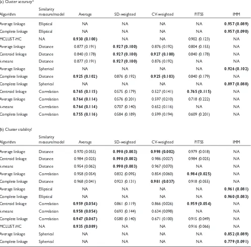
Completely synthetic data at low noise level

Table 2a,b shows selected results on cluster accuracy and cluster stability on the completely synthetic datasets with four simulated repeated measurements. Table 2a,b show results from average linkage, complete linkage and centroid linkage hierarchical algorithms, k-means, MCLUST-HC (a hierarchical model-based clustering algorithm from MCLUST) and IMM. Both single linkage and DIANA produce very low-quality and unstable clusters and their adjusted Rand indices are not shown. For each clustering approach, we produced six clusters (which is the number of classes). The results from CAST are not shown because the input parameter cannot be tuned to produce exactly six clus-ters in many cases. The FITSS column refers to the method of forcing repeated measurements into the same subtrees.

Because k-means is not hierarchical, its results are not avail-able (NA) under the FITSS column. Both centroid linkage hierarchical algorithm and k-means algorithm require the raw data matrix as input, so we cannot apply these two algo-rithms to cluster the posterior pairwise probabilities from the IMM approach.

In terms of cluster accuracy, the elliptical model of IMM pro-duced the highest level of agreement (adjusted Rand index = 0.957) with the six classes, and the hierarchical model-based clustering algorithm (MCLUST-HC) also produced clusters with high agreement (adjusted Rand index = 0.930) with the six classes. Within the same clustering algorithm, different similarity measures and different methods to deal with repeated measurements yield different cluster accuracy. For example, average linkage hierarchical algorithm produced more accurate clusters with Euclidean distance (variability-weighted or average over-repeated measurements) than correlation. The variability-weighted similarity approach produced more accurate clusters using SDs as the variability estimates than using the CVs. It is also interesting to note that SD-weighted correlation produced relatively low-quality clusters, whereas SD-weighted distance produced relatively accurate clusters. The FITSS approach of forcing repeated measurements into the same subtrees in hierarchical clus-tering algorithms does not yield high cluster accuracy.

In terms of cluster stability, most clustering approaches yield stable clusters (with average adjusted Rand indices above 0.900) except the spherical model of the IMM approach. This is because the spherical model assumes homogeneous variability for each gene across the experi-ments (which is not true on this synthetic data).

Completely synthetic data at high noise level

Tables 3a,b show the results on cluster accuracy and cluster stability on the completely synthetic data with four repeated measurements at high noise level. Even at a higher noise level, the elliptical model of IMM produced much more accurate clusters (average adjusted Rand index = 0.911 and 0.910 using average linkage or complete linkage) than all other approaches (SD-weighted distance and k-means pro-duced an average adjusted Rand index of 0.801). In general, the relative rankings of various clustering approaches at high noise level are similar to those at low noise level, except that the model-based hierarchical approach (MCLUST-HC) pro-duced less accurate clusters than the SD-weighted distance approach using the heuristically based algorithms.

(7)

distance approach produced substantial improvement in cluster quality over the approach of averaging over repeated measurements using the same algorithms at high noise level.

In terms of cluster stability (see Table 3b), the following three approaches yield average adjusted Rand index above 0.900: the elliptical model of the IMM approach; the

comment

reviews

reports

interactions

information

[image:7.609.57.555.125.614.2]

Table 2

Cluster accuracy and stability on the completely synthetic data with four repeated measurements at low noise level

(a) Cluster accuracy*

Similarity

Algorithm measure/model Average SD-weighted CV-weighted FITSS IMM

Average linkage Elliptical NA NA NA NA 0.957 (0.089)

Complete linkage Elliptical NA NA NA NA 0.957 (0.090)

MCLUST-HC NA 0.930 (0.100) NA NA 0.902 (0.123) NA

Average linkage Distance 0.877 (0.191) 0.927 (0.100) 0.876 (0.192) 0.804 (0.155) NA Centroid linkage Distance 0.840 (0.178) 0.927 (0.100) 0.927 (0.100) 0.840 (0.178) NA

k-means Distance 0.877 (0.191) 0.927 (0.100) 0.876 (0.192) NA NA

Average linkage Spherical NA NA NA NA 0.926 (0.102)

Complete linkage Distance 0.925 (0.102) 0.876 (0.192) 0.925 (0.103) 0.840 (0.179) NA

Complete linkage Spherical NA NA NA NA 0.897 (0.088)

Centroid linkage Correlation 0.765 (0.115) 0.575 (0.179) 0.527 (0.141) 0.765 (0.115) NA Average linkage Correlation 0.764 (0.114) 0.576 (0.201) 0.597 (0.210) 0.718 (0.222) NA

k-means Correlation 0.764 (0.114) 0.707 (0.140) 0.652 (0.116) NA NA

Complete linkage Correlation 0.755 (0.116) 0.584 (0.189) 0.599 (0.194) 0.609 (0.201) NA

(b) Cluster stability†

Similarity

Average linkage Distance 0.970 (0.055) 0.998 (0.003) 0.998 (0.002) 0.979 (0.018) NA Centroid linkage Distance 0.984 (0.025) 0.998 (0.002) 0.986 (0.027) 0.984 (0.025) NA

Average linkage Correlation 0.958 (0.054) 0.832 (0.095) 0.854 (0.060) 0.984 (0.025) NA Complete linkage Distance 0.968 (0.041) 0.923 (0.131) 0.981 (0.037) 0.918 (0.055) NA

Centroid linkage Correlation 0.959 (0.054) 0.861 (0.119) 0.866 (0.026) 0.959 (0.054) NA

*Each entry shows the average adjusted Rand index of the corresponding clustering approach with the six classes. We ran our experiments on five randomly generated synthetic datasets, and show the average results with the SD of the adjusted Rand index in brackets. A high average adjusted Rand index represents close agreement with the classes on average. †_{Each entry shows the average adjusted Rand index of the original clustering result with}

(8)

SD-weighted distance using average linkage and centroid linkage. It is interesting that the spherical model of the IMM approach produces unstable clusters at both high and low noise levels.

Yeast galactose data

[image:8.609.58.554.126.607.2]

Table 4a,b show selected results on cluster accuracy and cluster stability on real yeast galactose data. The true mean column in Table 4a refers to clustering the true mean data Table 3

Cluster accuracy and stability on the completely synthetic data with four repeated measurements at high noise level

Similarity

Complete linkage Distance 0.498 (0.113) 0.798 (0.144) 0.660 (0.098) 0.014 (0.030) NA Centroid linkage Distance 0.000 (0.000) 0.762 (0.113) 0.315 (0.156) 0.000 (0.000) NA Average linkage Distance 0.000 (0.000) 0.713 (0.217) 0.256 (0.071) 0.000 (0.000) NA

Average linkage Correlation 0.389 (0.151) 0.519 (0.159) 0.378 (0.081) 0.291 (0.130) NA Complete linkage Correlation 0.450 (0.122) 0.518 (0.159) 0.484 (0.156) 0.341 (0.112) NA Centroid linkage Correlation 0.358 (0.097) 0.261 (0.101) 0.215 (0.096) 0.358 (0.097) NA

(b) Cluster stability

Similarity

Average linkage Distance 0.208 (0.075) 0.932 (0.049) 0.812 (0.138) 0.381 (0.103) NA Centroid linkage Distance 0.211 (0.087) 0.920 (0.097) 0.779 (0.169) 0.211 (0.087) NA

Average linkage Correlation 0.721 (0.060) 0.782 (0.083) 0.692 (0.103) 0.855 (0.015) NA Complete linkage Distance 0.429 (0.105) 0.803 (0.159) 0.582 (0.083) 0.126 (0.025) NA Centroid linkage Correlation 0.731 (0.130) 0.497 (0.109) 0.430 (0.099) 0.731 (0.130) NA

*Each entry shows the average adjusted Rand index of the corresponding clustering approach with the six classes. We ran our experiments on five randomly generated synthetic datasets, and show the average results with the standard deviation of the adjusted Rand index in brackets. A high average adjusted Rand index represents close agreement with the classes on average. †_{Each entry shows the average adjusted Rand index of the original clustering}

(9)

(estimated with the error model suggested by Ideker et al. [24]) instead of clustering the repeated measurements. For each clustering approach, we produced four clusters (which is the number of functional categories).

The highest level of cluster accuracy (adjusted Rand index = 0.968 in Table 4a) was obtained with several algorithms: centroid linkage hierarchical algorithm with Euclidean dis-tance and averaging over the repeated measurements; hier-archical model-based algorithm (MCLUST-HC); complete linkage hierarchical algorithm with SD-weighted distance; and IMM with complete linkage. Clustering with repeated measurements produced more accurate clusters than clus-tering with the estimated true mean data in most cases.

Table 4b shows that different clustering approaches lead to different cluster stability with respect to remeasured data. Similar to the results from the completely synthetic data, Euclidean distance tends to produce more stable clusters than correlation (both variability-weighted and average over repeated measurements). Clustering results using FITSS were less stable than the variability-weighted approach and the averaging over repeated measurements approach.

SD produced more accurate and more stable clusters than CV in the variability-weighted similarity approach, especially when Euclidean distance is used. In addition, the model-based approaches (MCLUST-HC and IMM) produced rela-tively accurate and stable clusters on this data.

Effect of different numbers of repeated measurements

To study the effect of different numbers of repeated measure-ments on the performance of various clustering approaches, we generated completely synthetic data with different numbers of simulated repeated measurements for each data point. Specifically, we generated 1, 4, or 20 repeated measure-ments at both the low and high noise levels. The quality of clustering results on datasets with higher numbers of repeated measurements is usually higher (Table 5). For example, using the same algorithms and same similarity measures cluster accuracy is considerably improved with synthetic datasets of four repeated measurements relative to datasets with no repeated measurement. With 20 repeated measurements, Euclidean distance is less sensitive to noise, and the SD-weighted distance approach produces comparable cluster accuracy to IMM. This is probably because the variability esti-mates computed over 20 repeated measurements are much more robust than those with four repeated measurements. Nevertheless, the elliptical model of IMM consistently pro-duced the most accurate clusters over different numbers of simulated repeated measurements and different noise levels.

Discussion

We showed that different approaches to clustering array data produce clusters of varying accuracy and stability. We

also showed that the incorporation of error estimates esti-mated from repeated measurements improves cluster quality. We also show that the elliptical model of IMM con-sistently produced more accurate clustering results than other approaches using both real and synthetic datasets, especially at high noise levels. The variability-weighted approach tends to produce more accurate and more stable clusters when used with Euclidean distance than the simple approach of averaging over the repeated measurements. In addition, the SD-weighted distance usually produces more accurate and more stable clusters than the CV-weighted dis-tance. In general, the results are consistent across both real and synthetic datasets.

Limitations

In all the above results, we produced clustering results in which the number of clusters was set equal to the number of classes. In agglomerative hierarchical clustering algorithms (for example, average linkage), we successively merged clus-ters until the desired number of clusclus-ters, K, is reached, and considered the K subtrees as our K clusters, whereas in other algorithms the number of clusters was provided as input. A concern is that using a fixed number of clusters will force different classes into the same cluster owing to one or more outliers occupying a cluster. In such cases, the adjusted Rand index might improve with a larger number of clusters.

However, we chose to use a fixed number of clusters for several reasons. First, with the exception of the model-based algorithms, all other clustering algorithms (directly or indi-rectly) require the number of clusters as input. Even with the model-based algorithms, the number of clusters can only be estimated. In MCLUST-HC, the number of clusters can be estimated using a statistical score (see [29]). In the IMM approach, the number of clusters can be estimated from the posterior distribution of clustering results (see [18]). Second, it is very difficult, if not impossible, to compare cluster quality over a range of different clustering algorithms when the number of clusters is not fixed. Finally, increasing the number of clusters does not always yield better clusters or higher Rand indices (data not shown).

There are also some limitations with the external criteria for the real datasets used in our empirical study. With the yeast galactose data, we used a subset of 205 genes, which contains many genes previously shown to be strongly co-regulated and which reflect four functional categories in the GO listings [23]. This subset of genes may be biased in the sense that they are not chosen entirely independently of their expres-sion patterns. In addition, there may be good biological reasons why some genes in the chosen set of 205 should not cluster into groups segregated by the GO classifications.

Distributions of variability-weighted similarity measures

The essence of the variability-weighted similarity approach is that the pairwise similarities take into account the variability

comment

reviews

reports

interactions

information

(10)

in repeated measurements. In an attempt to understand the effect of variability between repeated measurements on these similarity measures, we computed the correlation coeffi-cients between all pairs of genes in the yeast galactose data and plotted the distribution of the fraction of gene pairs against correlation coefficient by averaging over repeated

measurements and against SD-weighted correlation in Figure 2. The distribution of CV-weighted correlation is similar to that of SD-weighted.

[image:10.609.58.556.128.590.2]

Figure 2 shows that when SD is used in variability-weighted correlation, there are more gene pairs with correlation Table 4

Cluster accuracy and stability on yeast galactose data

Similarity

Algorithm measure/model Average SD-weighted CV-weighted FITSS True mean IMM

Centroid linkage Distance 0.968 0.849 0.802 0.968 0.159 NA

MCLUST-HC NA 0.968 NA NA 0.968 0.806 NA

Complete linkage Distance 0.957 0.968 0.957 0.643 0.695 NA

Complete linkage Spherical NA NA NA NA NA 0.968

Complete linkage Elliptical NA NA NA NA NA 0.968

Centroid linkage Correlation 0.942 0.807 0.753 0.942 0.942 NA

k-means Correlation 0.871 0.640 0.827 NA 0.897 NA

Average linkage Spherical NA NA NA NA NA 0.897

Average linkage Elliptical NA NA NA NA NA 0.897

Average linkage Distance 0.858 0.858 0.847 0.869 0.159 NA

Average linkage Correlation 0.866 0.817 0.841 0.865 0.857 NA

k-means Distance 0.857 0.857 0.767 NA 0.159 NA

Complete linkage Correlation 0.677 0.724 0.730 0.503 0.744 NA

(b) Cluster stability†

Similarity

Complete linkage Elliptical NA NA NA NA 0.998

Complete linkage Spherical NA NA NA NA 0.991

Average linkage Distance 0.820 0.985 0.914 0.650 NA

MCLUST-HC NA 0.963 NA NA 0.916 NA

Complete linkage Distance 0.927 0.937 0.830 0.441 NA

Centroid linkage Distance 0.893 0.924 0.841 0.893 NA

Average linkage Spherical NA NA NA NA 0.923

k-means Distance 0.905 0.867 0.798 NA NA

Average linkage Elliptical NA NA NA NA 0.895

Centroid linkage Correlation 0.889 0.758 0.644 0.889 NA

Average linkage Correlation 0.842 0.842 0.855 0.828 NA

k-means Correlation 0.799 0.709 0.781 NA NA

Complete linkage Correlation 0.655 0.700 0.666 0.577 NA

(11)

coefficients around 0 and fewer gene pairs with correlation coefficients near 1. Figure 3 shows the distribution of Euclid-ean distance by averaging over the repeated measurements and the SD-weighted distance on the same data. There are more gene pairs with distance close to zero when variability estimates are used to weigh distance. This shows that weigh-ing similarity measures with variability estimates produces more conservative estimates of pairwise similarities.

Moreover, we showed that on average, variability-weighted similarity measures (both correlation and distance) computed from repeated measurements produced pairwise similarities closer to the true similarity than similarity measures

computed from data with no repeated measurement. In our simulation experiment, we computed the true pairwise cor-relation and distance between all pairs of genes on the esti-mated true mean yeast galactose data (using the error model

in Ideker et al. [24]). We also computed the

variability-weighted correlation and distance between all pairs of genes

comment

reviews

reports

interactions

information

[image:11.609.314.556.89.280.2]

Table 5

Cluster accuracy on the completely synthetic datasets with different numbers of repeated measurements

Number Similarity

of repeated measure/

SD-measurements Noise model Average weighted IMM

1 Low Correlation 0.680 NA NA

1 Low Distance 0.789 NA NA

1 Low Spherical NA NA 0.804

1 Low Elliptical NA NA 0.804

1 High Correlation 0.259 NA NA

1 High Distance 0.000 NA NA

1 High Spherical NA NA 0.395

1 High Elliptical NA NA 0.395

4 Low Correlation 0.764 0.576 NA

4 Low Distance 0.877 0.927 NA

4 Low Spherical NA NA 0.926

4 Low Elliptical NA NA 0.957

4 High Correlation 0.389 0.519 NA

4 High Distance 0.000 0.713 NA

4 High Spherical NA NA 0.589

20 Low Correlation 0.854 0.701 NA

20 Low Distance 0.891 0.964 NA

20 Low Spherical NA NA 0.962

20 Low Elliptical NA NA 0.957

20 High Correlation 0.602 0.651 NA

20 High Distance 0.590 0.819 NA

20 High Spherical NA NA 0.688

Cluster accuracy on the completely synthetic data with different numbers of repeated measurements and different noise levels using average linkage hierarchical clustering algorithm. For each number of repeated

measurements and noise level, the highest average adjusted Rand index is shown in bold. As we generated five random synthetic datasets, the results shown are averaged over five synthetic datasets.

Figure 2

Distribution of the fraction of gene pairs against correlation coefficient. Correlation coefficients are computed from averaging over repeated measurements and using SD over repeated measurements as weights on the yeast galactose data. There are more gene pairs with correlation coefficients around 0 and fewer gene pairs with correlation coefficients near 1 when SD-weighted correlation is used.

Correlation coefficient

Fraction of gene pairs

−

0.92 ₋0.79 ₋0.67 ₋0.54 ₋0.41 ₋0.28 ₋0.15 ₋0.03 0.10 0.23 0.36 0.49 0.61 0.74 0.87 1.00

0.00 0.01 0.02 0.03 0.04 0.05 0.06 0.07 0.08

Average over repeated measurements

[image:11.609.56.296.129.509.2]

SD-weighted

Figure 3

Distribution of the fraction of gene pairs against Euclidean distance. Euclidean distances are computed from averaging over repeated measurements and using SD over repeated measurements as weights on the yeast galactose data. There are more gene pairs with Euclidean distances near 0 when SD-weighted distance is used.

Euclidean distance

Fraction of gene pairs

0.00 0.10 0.20 0.30 0.40 0.50 0.60 0.70 0.80 0.90 1.00 1.10 1.20 1.30 1.40 1.51

0.00 0.02 0.04 0.06 0.08 0.10 0.12 0.14 0.16 0.18

Average over repeated measurements

[image:11.609.314.555.359.575.2]

(12)

on the synthetic remeasured data generated from the same error parameters and mean intensities as the yeast galactose data. In addition, we computed correlation and distance using only one of the repeated measurements in the remea-sured data. Then, we compared the average deviation of the variability-weighted similarity measures from the truth, and the average deviation of the similarity measures on the data with no repeated measurements to the truth (see Materials and methods for detailed results).

Modified variability-weighted approach

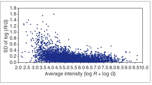
One of the drawbacks of the current definitions of the variabil-ity-weighted similarity approach is that only noisy experi-ments are down-weighted, whereas noisy genes are not. Suppose we have a dataset in which some genes are noisier than others, but the noise levels across the experiments stay relatively constant. In this scenario, the variability-weighted approach would not improve cluster quality. Genes expressed at low levels are frequently expressed at low levels across all experiments and usually have higher variability (see Figure 4). Hence, unless we filter out low-intensity genes, the weighting

methods developed by Hughes et al.([2] and see Materials

and methods) will not down-weight these genes. We attempted to correct for this effect by removing the normaliz-ing factor in the definition of variability-weighted distance (see Materials and methods for mathematical definitions). This improved the clustering accuracy when Euclidean dis-tance was used. However, we did not see improvement using this method with correlation as the similarity measure.

Conclusions

Our work shows that clustering array data with repeated measurements can significantly improve cluster quality, especially when the appropriate clustering approach is applied. Different clustering algorithms and different methods to take advantage of repeated measurements (not

surprisingly) yield different clusters with different quality. In practice, many clustering algorithms are frequently run on the same dataset and the results most consistent with previous beliefs are published. A better approach would be to use a clustering algorithm shown to be the most accurate and stable when applied to data with similar signal-to-noise and other characteristics as the data of interest. In this work, we ana-lyzed both real and completely synthetic data with many algo-rithms to assess cluster accuracy and stability. In general, the model-based clustering approaches produce higher-quality clusters, especially the elliptical model of the IMM. In particu-lar, the higher the noise level, the greater the performance dif-ference between the IMM approach and other methods.

For the heuristically based approaches, average linkage hier-archical clustering algorithm combined with SD-weighted Euclidean distance also produces relatively stable and accu-rate clusters. On the completely synthetic data, we showed that the infinite mixture approach works amazingly well with only four repeated measurements, even at high noise levels. The variability-weighted approach works almost as well as the IMM with 20 repeated measurements. From our results on the synthetic data, we showed that there is significant improvement in cluster accuracy from one to four repeated measurements using IMM at both low and high noise levels (Table 5). However, there is no substantial improvement in cluster accuracy from 4 to 20 repeated measurements with the IMM approach (Table 5).

There are many possible directions of future work, both methodological and experimental. Because the elliptical model of IMM produces very high-quality clusters, it would be interesting to develop a similar error model in the finite model-based framework on MCLUST and to compare the performance of the finite versus infinite mixture approaches. Another practical methodological development would be to incorporate the estimation of missing data values into the model-based approaches. It would also be interesting to develop other variability-weighted similarity measures that would down-weight both noisy genes and noisy experiments.

In terms of future experimental work, we would like to eval-uate the performance of various clustering algorithms on array data with repeated measurements on more real datasets. One of the difficulties we encountered is that there are very few public datasets that have both repeated mea-surements and external criteria available. We would greatly appreciate it if readers would provide us with access to such datasets as they become available.

Materials and methods

Datasets

Yeast galactose data

Ideker et al.[22] studied galactose utilization in yeast using

[image:12.609.55.299.544.681.2]

cDNA arrays by deleting nine genes on the galactose utilization Figure 4

Distribution of error plotted against intensity. The SDs over the log ratios from repeated measurements are plotted against the average intensities over repeated measurements in a typical experiment on the yeast galactose data.

1.8 1.6 1.4 1.2 1.0 0.8 0.6

2.0 2.5 3.0

SD of log (

R

/

G

)

3.5 4.0 4.5 5.0 5.5

Average intensity (log R + log G)

6.0 6.5 7.0 7.5 8.0 8.5 9.0 9.510.0 0.4

(13)

pathway in the presence or absence of galactose and raffi-nose. There are a total of 20 experiments (nine single-gene deletions and one wild-type experiment with galactose and raffinose, nine deletions and one wild-type without galactose and raffinose). Four replicate hybridizations were performed for each experiment. We used a subset of 205 genes from this data, whose expression patterns reflect four functional categories in the GO [23].

Synthetic remeasured cDNA data

Let xijrand yijrbe the fluorescent intensities of the two

chan-nels (fluorescent dyes) for gene i, experiment jand repeated

measurement r, where i=1, …, G, j=1, .., E, r=1, .., R. For

the yeast galactose data, G is approximately 6,000, E is 20

and R is 4. Ideker et al. [24] proposed an error model for

replicated cDNA array data in which the observed fluores-cent intensity levels are related to their true expression levels by the following model:

x_ijr= ␮_xij+ ␮_xij⑀_xijr+ ␦_xijr y_ijr= ␮_yij+ ␮_yij⑀_yijr+ ␦_yijr

where (␮xij, ␮yij) are the true mean intensity levels for gene i

under experiment jin the two channels. The multiplicative

error parameters in the two channels (⑀_xijr, ⑀_yijr) are assumed

to follow the bivariate normal distribution with mean 0, SDs

␴_⑀xj, ␴⑀yj and correlation ␳⑀j. Similarly, the additive error

parameters (␦_xijr, ␦_yijr) are assumed to follow the bivariate

normal distribution with mean 0, SDs ␴_␦_xj, ␴_␦_yjand

correla-tion ␳_␦_j. The gene-independent parameters (␴_⑀_xj, ␴_⑀_yj, ␳_⑀_j, ␴_␦_xj,

␴␦yj, ␳␦j) and the gene-dependent parameters (␮xij, ␮yij),

where i= 1, …, G and j=1, …, E, are estimated by maximum

likelihood [24].

Using this error model, we estimate the true expression intensities for each gene and the gene-independent parame-ters for each of the 20 experiments in the yeast galactose

data. From the gene independent parameters (␴_⑀_xj, ␴_⑀_yj, ␳_⑀_j,

␴␦xj, ␴␦yj, ␳␦j), we generate random (⑀xijr, ⑀yijr) and (␦xijr, ␦yijr)

from the bivariate normal distributions. Hence, we can gen-erate random remeasured data (and log ratios) using the

estimated true mean intensities (␮xij, ␮yij).

Completely synthetic data

The completely synthetic datasets consist of 400 data points

(genes), 20 attributes (experiments) and 6 classes. Let ␾(i,j)

be the artificial pattern of gene iand experiment j before error

is added, and suppose gene ibelongs to class k. Four of the six

classes follow the periodic sine function (␾(i,j) = sin (2␲j/10 –

wk)), and the remaining two classes follow the non-periodic

linear function (␾(i,j) = j/20 or ␾(i,j) = -j/20), where i= 1, 2, 3,

…, 400, j= 1, 2, 3, …, 20, k= 1, 2, 3, 4 and w_kis a random

phase shift between 0 and 2_␲. Let X(i,j,r) be the error-added

value for gene i, experiment j and repeated measurement

r. Let the randomly sampled error be ␴ij for gene i and

experiment j, and X(i,j,r) is generated from a random normal

distribution with mean equal to ␾(i,j), and SD equal to ␴_ij.

We define the signal-to-noise ratio of a synthetic dataset to be the ratio of the range of signals (in our case, 1-(-1) = 2) to the average sampled error. For the completely synthetic data shown in Figure 1a,b, the signal-to-noise ratios are 14.3 and 2.5 respectively.

Missing data

The yeast galactose dataset [22] contains approximately 8% of missing data values. There are many possible sources of missing data values, for example, low signal-to-noise ratios, dust or scratches on slides. As the current versions of MCLUST [30] and the IMM implementation [18] do not handle missing data values, we impute the missing data values. We experimented with two imputation methods, namely model-based multiple imputation [31] as imple-mented in Splus, and weighted k-nearest neighbors (KNNim-pute) [32]. We found that data after KNNimpute produce higher-quality clusters than data after model-based multiple imputation. Therefore, we applied KNNimpute to the yeast galactose data before applying the model-based approaches.

Notations and similarity measures

Suppose there are Ggenes, Eexperiments, and Rrepeated

measurements. Denote the measured expression level from

repeated measurement r of gene gunder experiment e as

X_ger, where g=1, …, G, e= 1, …, Eand r= 1, …, R. Let Dbe

the raw data matrix such that D(g,e) represents the average

expression level over Rrepeated measurements for gene g

under experiment e, that is,

⌺

R

r=1Xger/R,

where g= 1, …, G, e = 1, …, E. The correlation coefficient

between a pair of genes iand j(i,j= 1, .., G) is defined as

⌺

E

e=1(D(i,e) - ␮i)(D(j,e) - ␮j)

␳ij= ——————————————————————_{———————————————————}

e

⌺

E=1(D(i,e) - ␮i) 2

⌺

E

e=1(D(j,e) - ␮j) 2

where

␮i=

⌺

E e=1 E

————D(i,e)

is the average expression level of gene iover all E

experi-ments. The Euclidean distance between a pair of genes iand

j(i,j= 1, .., G) is defined as

————————————–— dij=

—1_E

⌺

E e=1

(D(i,e) - (D(j,e))2 .

comment

reviews

reports

interactions

information

(14)

Similarly, we can define correlation and Euclidean distance between a pair of experiments by swapping the positions of the gene and experiment indices.

Variability-weighted similarity measures

Hughes et al. [2] defined error-weighted similarity measures

that weight expression values with error estimates such that expression values with relatively high errors are

down-weighted. Let ␴_ge be the error estimate of the expression

level of gene gunder experiment e, where g= 1, …, Gand e= 1,

…, E. The error-weighted correlation between a pair of genes

iand jis defined as

(D(i,e) - ␮~_i) (D(j,e) - ␮~_j)

⌺

E

e=1

—————–—— —————–——_␴

ie ␴je

␳~ij= ————————————————————————————

—————————————————————————— D(i,e) - ␮~i

2

D(j,e) - ␮~i

⌺

eE=1

—————–—

⌺

E

e=1

—————–——

2

␴ie ␴je

where

␮~

i=

⌺

E e=1 ———␴ie

D(i,e)

/

⌺

E e=1 ———␴ie

1

is the weighted average expression level of gene i. Similarly, the error-weighted Euclidean distance [2] is defined as

———————————————————————

(D(i,e) -D(j,e))2 1

d~ij=

⌺

E e=1

–––––––––––––––

/

⌺

E e=1

–––––––– .

␴ie2+ ␴je2 ␴ie2+ ␴je2

In our empirical study, variability estimates are used instead of error estimates. In particular, we use either the SD or CV

over the Rrepeated measurements as ␴ge. These

variability-weighted similarity measures serve as inputs to many clus-tering algorithms.

Modified variability-weighted distance

The above definitions of variability-weighted correlation and distance down-weight noisy experiments in computing the pairwise similarity, but would not work in the case of noisy

genes. Consider two pairs of genes, (X, Y) and (W, Z), such

that D(X,e) = D(W,e) and D(Y,e) = D(Z,e) and ␴_Xe =

␴Ye<<␴We= ␴Ze for all experiments e. In other words, the

expression patterns of gene Xand gene Ware identical, so

are the patterns of gene Yand gene Z. The levels of noise (or

variability) are constant across all the experiments for each

pair of genes, but genes (W,Z) are much more noisy than

genes (X,Y). Using the above definitions of

variability-weighted similarity, ␳~XY= ␳~WZ and d

~

XY= d

~

WZ. Intuitively,

one would expect the pairwise similarity between genes

(W,Z) to be lower than that of genes (X,Y) because genes

(W,Z) are more noisy. We experimented with a modified

def-inition of variability-weighted distance by removing the scaling factor in the denominator:

————————————————

(D(i,e) -D(j,e))2

d~_ijⴕ=

⌺

E e=1

–––––––––––––––

/

E

␴ie2+ ␴je2

This modified definition tends to give slightly better clusters (see Additional data files and [33]).

Clustering algorithms

Agglomerative hierarchical algorithms

In agglomerative hierarchical clustering algorithms [5], each object is initially assigned to its own cluster (subtree), and the number of initial clusters is equal to the number of objects. Similar clusters (subtrees) are successively merged to form a dendrogram. In each merging step, the number of clusters (subtrees) is reduced by one. This merging process is repeated until the desired number of clusters, K, is pro-duced. The objects in these K subtrees form the resulting K clusters, and the hierarchical structures of the subtrees are ignored.

Different definitions of cluster similarity yield different clus-tering algorithms. In a single linkage hierarchical algorithm, the cluster similarity of two clusters is the maximum similar-ity between a pair of genes, one from each of the two clus-ters. In a complete linkage hierarchical algorithm, the cluster similarity is defined as the minimum similarity between a pair of genes, one from each of the two clusters. In an average linkage hierarchical algorithm, the cluster simi-larity of two clusters is the average pairwise simisimi-larity between genes in the two clusters. In a centroid linkage hier-archical algorithm, clusters (subtrees) are represented by the mean vectors of the clusters, and cluster similarity is defined as the similarity between the mean vectors.

k-means

K-means [7] is a classic iterative clustering algorithm, in which the number of clusters is an input to the algorithm. Clusters are represented by centroids, which are cluster centers. The goal of k-means is to minimize the sum of dis-tances from each object to its corresponding centroid. In each iteration, each gene is assigned to its closest centroid. After the gene reassignment, new centroids are computed. The steps of assigning genes to centroids and computing new centroids are repeated until no genes are moved between clusters. In our implementation, we use the clusters from average linkage hierarchical algorithm to compute initial centroids to start k-means.

MCLUST

(15)

MCLUST also includes a clustering function (hcVVV) that uses model-based hierarchical clustering to initialize the EM algorithm. Because the current version of MCLUST does not have any mechanism to incorporate repeated measure-ments, but does allow initializations at nontrivial partitions, we initialize the hierarchical model-based algorithm with subtrees containing repeated measurements. We use the most general model (unconstrained) for hierarchical cluster-ing, which allows each cluster to have different volume, ori-entation and shape. This approach is abbreviated as MCLUST-HC.

IMM

The IMM approach uses a Gibbs sampler to estimate the posterior pairwise probabilities. The Gibbs sampler requires two sets of parameters for input: initialization parameters (random seed and the initial number of mixture compo-nents) and convergence parameters (initial annealing coeffi-cient, the rate of ‘cooling’ and the ‘burn-in’ period). A posterior distribution with multiple peaks could result in Gibbs samplers’ inability to escape from a suboptimal peak. The role of the annealing coefficient [34] is to flatten the posterior distribution of clustering results and thus alleviate the difficulty in transitioning between high-probability regions that are separated by regions of low probability, which is a common problem of Gibbs samplers in general [35]. Burn-in corresponds to the number of initial iterations that the Gibbs sampler takes to converge to the posterior dis-tribution, and the burn-in iterations are not used in calculat-ing posterior pairwise probabilities. We tuned the convergence parameters by running independent samplers with different initialization parameters, and chose the set of convergence parameters that yielded the highest correlation between pairwise probabilities over different runs and over different random perturbations of the data. Using this simple principle, we identified a single combination of the annealing parameters that resulted in excellent convergence in all datasets we analyzed, including some not reported in this paper. This combination consisted of the initial anneal-ing coefficient of 0.01, rate of coolanneal-ing of 0.999 and the burn-in of 10,000 iterations. For burn-investigators analyzburn-ing their own data, we suggest that they run at least five independent Gibbs samplers with this combination of parameters from five different initial numbers of clusters and establish that all five converge to the same posterior distribution. This can be done by calculating correlation between posterior pairwise probabilities from different runs. Alternatively, the adjusted Rand index can be used for comparing clustering results generated by different runs of the Gibbs sampler. If the cor-relations or adjusted Rand indices suggest that all five sam-plers did not converge to the same solution, investigators should try increasing the annealing coefficient (to say 0.9995) and the burn-in number of iterations (to say 20,000), and repeat the process. The Readme.txt file that accompanies the IMM software describes these parameters in detail.

CAST

The cluster affinity search technique (CAST) [21] is an itera-tive algorithm, in which objects are added to or removed from the current cluster until there are no more similar objects to be added and no more dissimilar objects to be removed. At this point, the current cluster is assumed to be done. A new cluster is started and the iterative process of adding and removing objects is repeated until all objects are assigned to clusters. The inputs to the algorithm include the pairwise similarities and a parameter that indirectly controls the number of clusters.

DIANA

DIANA [20] is a hierarchical divisive clustering algorithm, in which we start with all objects in one cluster. In each step, clusters are successively split to form two clusters until the desired number of clusters is reached. The cluster with maximum diameter (maximum pairwise dissimilarity) is split in each step. Let us call this the current cluster. The most dissimilar element in the current cluster is identified to start a new cluster. An object in the current cluster is moved to the new cluster if the average similarity with the new cluster is higher than that with the current cluster.

Completely synthetic data with different numbers of repeated measurements

Table 5 shows some selected results produced using average linkage hierarchical algorithm on the completely synthetic data over varying numbers of repeated measurements and different noise levels. In general, increasing the number of repeated measurements increases cluster accuracy (average adjusted Rand index with respect to the six classes). The elliptical model of IMM produced superior quality of clus-ters, especially at high noise levels.

Simulation experiment: variability-weighted similarity

We computed the true pairwise correlation and Euclidean dis-tance between all pairs of genes on the estimated true mean yeast galactose data. Denote the correlation between

esti-mated true means for gene iand gene jas ␳ijtrue. We generated

synthetic re-measured datasets using the same error parame-ters and true mean intensities of the yeast galactose data. Let

the variability-weighted correlation for gene iand gene jbe

␳

~

ijk, and the correlation computed using only one of the

repeated measurements, r(no repeated data) be ␳_ijkr_{, where}_k

is one of the randomly generated synthetic remeasured data.

The column |␳~- ␳true_{| in Table 6 shows the average of |}_␳~

ijk

-␳ijtrue| over all pairs of genes i, j, and all randomly remeasured

datasets k, while the column |␳r_-_␳true_{| shows the average of}

|␳ijkr - ␳ijtrue|over all pairs of genes i, j, all randomly

remea-sured datasets k, and all repeated measurements r. The

cor-responding results using distance are also shown in Table 6, which shows that on average the variability-weighted simi-larities are closer to the ‘truth’ than simisimi-larities computed from data with no repeated measurement.