Share valuation : resolving the negative
earnings puzzle
Fox, RP and Huruva, F
Title
Share valuation : resolving the negative earnings puzzle
Authors
Fox, RP and Huruva, F
Type
Conference or Workshop Item
URL
This version is available at: http://usir.salford.ac.uk/34680/
Published Date
2015
USIR is a digital collection of the research output of the University of Salford. Where copyright
permits, full text material held in the repository is made freely available online and can be read,
downloaded and copied for noncommercial private study or research purposes. Please check the
manuscript for any further copyright restrictions.
Share valuation: resolving the negative earnings
puzzle
Fox, R. P., and Huruva, F.
January 8, 2015
This paper presents a resolution of the apparently illogical observation in a number of papers that higher losses are associated with higher share valuations. We create conditional distributions from a sample of 42,857 firm years on the London Stock Exchange and show that the relationship is illusory. We argue that our model is better aligned with the concept of market efficiency and the problem of differentiating between observations and expectations. More generally, the model developed here can be applied to all studies that seek to explain market prices.
A number of studies (Ashton et al., 2003; Burgstahler and Dichev, 1997; Collins et al., 1999; Darrough and Ye, 2007; Hand, 2000; Jiang and Stark, 2013) observe high market values for high loss making firms. The problem is most clearly expressed by Jiang and Stark (2013) who make the following observation: ”The negative relationship between earnings and market value for loss-making firms is a puzzle because it is counter-intuitive, higher losses leading to higher market values does not make intuitive economic sense.” (p.113) This note offers a resolution of this apparent puzzle that is of interest to all studies seeking to relate market measures to accounting and economic variables.
THE PUZZLE DEFINED
The importance of accounting income to share prices has been well estab-lished in the literature since Ball and Brown (1968). A simple model of market value can therefore be expected to be strongly related to earnings. A basic version by Jiang and Stark (2013) is:
M Vt=a+bEt+BVt+εt (1)
where M V = market value, BV = book value of equity and E = net income to shareholders. Both Burgstahler and Dichev (1997) and Ashton et al. (2003)) apply an equivalent model using book value as a deflator:
M V /BVt=a+bE/BVt+εt (2)
for low earnings intervals are significantly negative . . . one explanation might be that. . . more negative values of E/BV may be empirically associated with actions which have been taken to improve E/BV in subsequent years and which are already reflected in higher market values” (p.203). This approach was devel-oped by Darrough and Ye (2007) who add ”value drivers” such as non-recurring charges, R&D, growth strategy and sustainability. They eliminate the relation-ship between negative earnings and market value with the major substitutes being R&D and intangible assets. These findings were tested on UK data by Jiang and Stark (2013) using various deflators and a wider set of explanatory variables. They failed to find a robust resolution and observe that there is: ”a higher degree of contextualisation of the loss-making firm valuation model” (p.123). On reflection, it should not be too surprising that separate modelling of a sub-sample of the earnings spectrum should prove to be unstable.
It therefore remains curious that empirical testing of equation 2 should pro-duce results that seem so theoretically appealing when earnings are positive and yet so unappealing when earnings are negative.
A REANALYSIS
It is understood in equations 1 and 2 that earnings represents expected earnings. Hence both market value and earnings are expectations about the future. One of the strongest findings in finance arising from weak form market efficiency tests is that share prices follow a martingale; information is randomly better or worse than expected. Therefore, the current price is taken as the best estimate of market expectations Capinski and Zastawniak, 2011, p.161). It is traditional to assume that the same reasoning can be applied to the explanatory variables. This is a convenient assumption to make, as current earnings can then be taken as best estimates of expected earnings. Unlike share prices, however, there is no theoretical argument to support this assumption. As the original paper (Samuelson, 1965) makes clear, explanatory variables may follow a pattern. The value of the pattern is discounted into the share price and information is information about changes to the expectation of the pattern. The product life cycle is one such example and both Burgstahler and Dichev (1997) and Darrough and Ye (2007) are in effect suggesting patterned earnings of ”non capitalized expenditure today - profit tomorrow”. It seems reasonable to assume that all firms with high value and high losses have such patterned expectations but most firms are not in that position. Indeed a martingale process might well be an adequate assumption for many if not most firms. Revisiting equation 2 and making expectations explicit, we have:
M V /BVi,t=a+bE/BVi,t+εi,t (3)
We agree with the conclusion of Jiang and Stark (2013) that the attempts to replace negativeEiwith variables that measureEiare insufficiently robust. We
from expectations will obviously occur and are part of the financial language; thus, a ”windfall profit” and ”writing off exceptional items” and more gener-ally, patterns where the current earnings presage higher returns in the future are all allowable. Note that this does not imply a normal distribution. We nevertheless expect for the market as a whole, earnings to be frequently close to expectations. If those expectations vary with market value, then we would expect that relationship to be positive as in equation 3. We therefore take a Bayesian view and examine earnings conditioned on market value to determine the expectation:
M V /BV =a+bE/BV|M V /BV +ε (4) This is a three stage process. Firstly, examine the distributions of
E/BV|M V /BV for varying levels ofM V to see if there is a concept of centrality in the distribution (typically a single peak triangular distribution). Secondly, measure the central point E/BV|M V /BV for all distributions conditioned on value ranges ofM V /BV, note that expectation is simply a measure of centrality here. Outliers, from whatever cause, need not influence such estimation. This is a more consistent methodology, since if outliers are regarded as not including earnings in valuation, then it seems contradictory to then include such earn-ings in a measure of market expectation. Thirdly, regress or more simply plot E/BV|M V /BV on M V /BV to examine the relationship. As we know that market values are valued efficiently using the whole of the public information set, it can be inferred that a true outlier of the conditional distribution is by im-plication responding to elements of the information set other than earnings. In this way, the martingale assumption has been dropped as we no longer assume that current earnings are expectations.
The relationship between an individual earnings observation and its expecta-tion is by this analysis probabilistic to which Bayes theorem applies, assuming a uniform prior:
P r(M V /BVk|E/BVj) =
P r(E/BVj|M/BVk)
P
k
P r(E/BVj|M/BVk)
(5)
Such an approach would not be of particular interest as no serious attempt to value a firm would just use earnings. In Bayesian terms the uniform prior will, rather like ceteris paribus, ignore much that is relevant.
EMPIRICAL TESTING
The overall purpose of testing is firstly to validate our sample with respect to previous studies. This we do by following the methodology of previous pa-pers (Burgstahler and Dichev, 1997; Ashton et al., 2003) as in equation 2, and test for the finding of a positive relationship between losses and market value. Then we examine earnings conditioned on market value to determine expected values. Finally, we examine the relation between expected earnings conditioned on market values and market values. The concern here is limited to resolving the puzzle by reformulating equation 2, our analysis is therefore to a sufficient level though our methodology indicates how further research might develop.
The database consisted of 42,857 firm years quoted on the London Stock Ex-change from 1988 to 2012 as stored on Datastream. We followed the definitions of Ashton et al. (2003) who use the same database. Earnings are defined as net income before extraordinary earnings (item 625); book value was defined as common shareholders equity less net intangible assets (item 305 - 344) which is in effect the equity claim on tangible assets, a definition prompted by the claim that such a value represents adaptation value for shareholders (Ashton et al., 2003). In supplementary tests we found that the inclusion or omission of intangible assets did not affect the results. Market value was taken as 100 days after the year end date to get a roughly contemporaneous valuation with the accounting data. A common observation in papers is that the results are not affected by different timings of share dates (e.g. Fama and French (1992)). Data not considered were firm years reporting book values less than £1,000 thus excluding negative M/BVs and very small book values that would poten-tially report extreme ratios. We are aware of criticisms of Datastream (Ince and Porter, 2006) but point out that with the exception of eliminating de-listed quotes, this paper does not deal with the issues addressed by Ince and Porter (2006). Measurement error will nevertheless always be present. An important feature of this approach is that market expectation is defined as the peak of a distribution and not necessarily the first moment. Extreme results due to measurement error need not influence expectations, the main requirement is therefore that errors are not systematic.
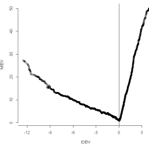
Figure 1: Plot of running medians of groups of 500 ordered by E/BV
To further validate our sample, we applied equation (2) and and compared the results with previous papers, in particular, Burgstahler and Dichev (1997), Ashton et al. (2003) and Darrough and Ye (2007). The sample was ordered by E/BV and plotted againstM/BV by creating running medians of both variables with a span of 5001as in figure 1. The plot shows a remarkably similar pattern
to previous papers2. There is a strong negative tail made up of 27% of the sample that reveals the negative relationship that is the basis of the puzzle. The curvature noted in Ashton et al. (2003) and Burgstahler and Dichev (1997) seems to have disappeared, instead there is a remarkable linearity that extends even to the outliers. Using linear regression on non overlapping medians (R2 of
0.998), the slope of the positive valuations represents an annuity capitalisation rate of 7.9% ieM/BV is greater by a factor of 12.62. The reasonableness of these figures makes it all the more curious that there is such a large and apparently inexplicable negative tail that appears here to be more prominent than previous studies.
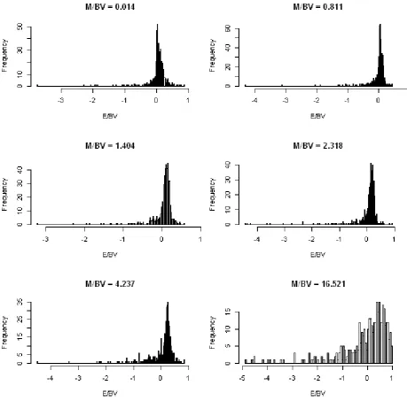
Figure 2: Histogram of groups of 500E/BVs ordered byM/BV
2 at regular intervals starting with the lowest M/BV. The histograms show reasonably well shaped distributions with large left (negativeE/BV) tails. It seems clear from figure 2 that there is a clustering ofE/BVs around what seems reasonable to regard as the typical value for a givenM/BV. The distributions also show that earnings are far less likely to overstate future expectations - the right hand tail. Together the distributions reflect the well established conser-vative measurement principles in accounting, it is interesting that this bias can be measured in this way.
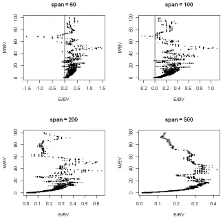
Figure 3: Plot of running medians of groups ordered byM/BV
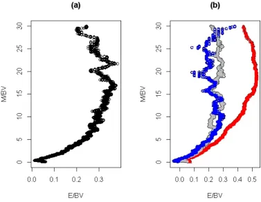
Figure 4: Expected E/BVs conditioned on M/BV (a)1988 to 2012; (b) red triangle 1988 to 1996, grey circle 1997 to 2005 and blue square 2006 to 2012
The third stage is to interpret the relationship. Taking spans of 500 for clarity, figure 4 shows that from aM/BV of about 0.4 (from more detailed graphs not reported here)to 7 there appears to be a relatively smooth relationship between E/BV andM/BV in the hypothesised direction. The slope of the line is 22.9 (using non overlapping medians, R2 of 94.4%) an implied discount factor of
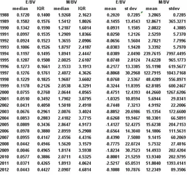
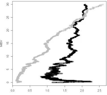
Figure 5: Negative E/BVs and Inter Quartile Ranges of E/BVs ordered by M/BV
later years. Whereas the studies of Burgstahler and Dichev (1997) and Ashton et al. (2003) cover the 1990’s and show, as here, that the relationship is smooth over the range, this cannot be said of later years. Further research is needed to determine what other factors affect market values at these higher market to book values.
incidence of negativeE/BVs. Thus the traditional approach that takesE/BV as an expectation would indeed trace an apparent positive relationship between losses and market value.
CONCLUDING DISCUSSION
The role of earnings in valuing a company is central to both theory and prac-tice. The observation in previous papers that higher losses appear to be related to higher market values is therefore an important anomaly. We have identi-fied the central problem as being the assumption that inter temporal earnings follow a martingale process thus equating observations with expectations. We have based our approach on the thesis that it is allowable for earnings not to be a martingale process (Samuelson, 1965). Exceptionally high valued firms ex-periencing losses can be expected to return to profitability for reasons that are more than just random variations around an expectation. By creating a series of distributions of earnings conditioned on market value and taking a measure of centrality of the distributions, we in effect detach observation from expectation. Taking the median as the centrality measure isolates outliers from the measure-ment process and is observably a more robust process (Table 1). As is normal with non parametric analysis (Fox, 2000) this relationship was observed rather than modelled. Tracing the market expectation ofE/BV for varying levels of M/BV we show that there are no negative E/BV expectations for reasonable samples sizes and hence no relationship between losses and market value. We find a remarkably linear positive relationship that is stable over time between earnings and market value between a M/BV of 0.4 and 7 which breaks down beyond this range. It seems eminently sensible to regard high levels and very low levels ofM/BV to be unrelated to either book value or earnings.
This more flexible interpretation of the role of an observation in the valuation process is very much in accord with what we observe. The huge financial centres across the world have share valuation as one of their central activities. The notion that it can be compressed into a traditional and fairly simple regression equation seems highly ambitious. Relating reported earnings to expectations is, as represented here, a far more complex, richer process.
Finally, our approach is not particular to earnings as an explanatory vari-able but is general to all varivari-ables that use historic values to model market prices. The particular relevance to earnings is the non normal nature of the inter temporal earnings for a significant number of firm years. This resulted in mis-identifying observations as expectations which was the source of the puzzle.
References
Ball, R. and Brown, P. (1968), ‘Empirical Evaluation of Accounting Income Numbers’,Journal of Accounting Research.
Burgstahler, D. C. and Dichev, I. D. (1997), ‘Earnings, Adaptation and Equity Value’,The Accounting Review72(2), 187–215.
Capinski, M. and Zastawniak, T. (2011),Mathematics for Finance: An Intro-duction to Financial Engineering, Springer.
Collins, D., Pincus, M. and Xie, H. (1999), ‘Equity Valuation and Negative Earnings: The Role of Book Value of Equity.’, The Accounting Review 74(1), 29– 61.
Darrough, M. and Ye, J. (2007), ‘Valuation of loss firms in a knowledge-based economy’,Review of Accounting Studies12, 61–93.
Fama, E. and French, K. R. (1992), ‘The Cross-Section of Expected Stock Re-turns’, Journal of FinanceXLVII(2), 427–465.
Fox, J. (2000),Nonparametric Simple Regression - smoothing scatterplots, Sage. Hand, J. (2000),Profits,Losses and Non Linear Pricing of Internet Stocks., In J. Hand and B.Lev Intangible Assets: Values, Measures and Risks, OUP:Oxford, UK.
Ince, O. S. and Porter, R. B. (2006), ‘Individual Equity Return Data from Thomson Datastream: Handle with Care’,The Journal of Financial Research XXIX(4), 463 – 479.
Jiang, W. and Stark, A. W. (2013), ‘Dividends, research and development ex-penditures and value relevance of book value forUK loss-making firms’, The British Accounting Review45, 112–124.