Potential based methodology for active sound control in three dimensional settings

Potential­based methodology for active 

sound control in three dimensional settings

Lim, H, Utyuzhnikov, SV, Lam, YW and Kelly, L

http://dx.doi.org/10.1121/1.4892934

Title

Potential­based methodology for active sound control in three dimensional 

settings

Authors

Lim, H, Utyuzhnikov, SV, Lam, YW and Kelly, L

Type

Article

URL

This version is available at: http://usir.salford.ac.uk/33319/

Published Date

2014

USIR is a digital collection of the research output of the University of Salford. Where copyright 

permits, full text material held in the repository is made freely available online and can be read, 

downloaded and copied for non­commercial private study or research purposes. Please check the 

manuscript for any further copyright restrictions.

Potential-based methodology for active sound control in three

dimensional settings

H. Lima)

I-Lab, Centre for Vision, Speech, and Signal Processing, University of Surrey, Guilford, Surrey GU2 7XH, United Kingdom

S. V. Utyuzhnikov

School of Mechanical, Aerospace and Civil Engineering, University of Manchester, Manchester M13 9PL, United Kingdom

Y. W. Lam and L. Kelly

Acoustics Research Centre, University of Salford, Salford, Greater Manchester, M5 4WT, United Kingdom

(Received 26 June 2012; revised 25 June 2013; accepted 1 August 2014)

This paper extends a potential-based approach to active noise shielding with preservation of wanted sound in three-dimensional settings. The approach, which was described in a previous publication [Limet al., J. Acoust. Soc. Am.129(2), 717–725 (2011)], provides several significant advantages over conventional noise control methods. Most significantly, the methodology does not require any information including the characterization of sources, impedance boundary conditions and sur-rounding medium, and that the methodology automatically differentiates between the wanted and unwanted sound components. The previous publication proved the concept in one-dimensional con-ditions. In this paper, the approach for more realistic conditions is studied by numerical simulation and experimental validation in three-dimensional cases. The results provide a guideline to the implementation of the active shielding method with practical three-dimensional conditions. Through numerical simulation it is demonstrated that while leaving the wanted sound unchanged, the developed approach offers selective volumetric noise cancellation within a targeted domain. In addition, the method is implemented in a three-dimensional experiment with a white noise source in a semi-anechoic chamber. The experimental study identifies practical difficulties and limitations in the use of the approach for real applications.VC _{2014 Acoustical Society of America.}

[http://dx.doi.org/10.1121/1.4892934]

PACS number(s): 43.50.Ki, 43.40.Sk, 43.55.Dt, 43.55.Br [BSF] Pages: 1101–1111

I. INTRODUCTION

Active sound control (ASC) is a technique for altering acoustic field to a wanted one in a given region of space by means of an active control boundary established by control-lable secondary sound sources. A typical problem formula-tion for ASC involves a domain to be protected from an external unwanted field (noise) by introducing special con-trol sources positioned on a boundary surface. The problem becomes more complicated if an internal wanted field is present and completely mixed up together with the noise in the domain. An obvious question in the case with wanted sound is how to obtain such separate cancellation of noise only from the total field measured at the boundary surface. Some available noise abatement techniques, for example, those developed by Kincaid et al.,1,2 require a detailed knowledge of the sources and nature of noise. A number of publications are also devoted to the optimization of the strength of the spatially distributed controls in order to mini-mize a quadratic pressure cost function.3,4

In recent years, different approaches have been sug-gested to realize real-time active noise control (see, e.g., Refs. 5–10). Most of them exploit the least mean square

(LMS) algorithm. Its application becomes problematic if the wanted sound component is present. In this case the use of LMS requires additional information on the wanted sound. For some applications it might be achieved via directional measurements.5,10 There have also been a few attempts to apply the virtual sensing and surface integral control to tackle this problem.8,9All of them are based on trying to pre-dict the wanted sound component and, therefore, are quite limited because the wanted ingredient cannot completely be separated from the total acoustic field.

The potential-based approach proposed can provide a convenient universal algorithm for the ASC problem in a quite general formulation associated with the unknown wanted sound and also unknown boundary conditions. The method requires no detailed knowledge of either the sound sources or boundary conditions, including reflection coeffi-cients that characterize the domain termination, to cancel out only the unwanted component. If the shape of the domain is complicated, the solution based on the developed technique allows us to choose a convenient boundary surface. The only input data needed for the control are the acoustic quantities of the field measured on the perimeter of the boundary surface. The measured quantities can pertain to be the overall field composed of both the adverse noise and wanted sound, and the methodology will automatically distinguish between the two.11,12In the current stage of the theoretical development,

a)_{Author to whom correspondence should be addressed. Electronic mail:}

the potential-based approach allows one to obtain the general solution to the ASC problem for arbitrary geometries, proper-ties of the medium, or boundary conditions.13,14

The method developed by Jessel and Mangiante,15,16 and Canevet,17hereby called the JMC method, also requires only information at the perimeter of the shielded domain for global noise absorption when only the unwanted noise is present in the protected domain. The main difference between the approaches based on the potential-based method and JMC is that only the former provides the advantages of preservation of the wanted sound and volumetric noise can-cellation through an entire shielded domain when the total field composed of both the wanted sound and noise is meas-ured at the boundary. One should note here that apart from the JMC, there are a number of other noise abatement techni-ques, which provide for the cancellation of noise in selected discrete18,19or directional areas.20In contrast to many other active noise control techniques, the potential-based ASC can naturally be realized in a discrete form12via the Difference Potential Method (DPM) formalism. From the standpoint of practical implementation, this is a clear advantageous because a realistic ASC system would require a discrete col-lection of control sources.

In Ref.21, the Difference Potential Method (DPM) was employed to solve a one-dimensional ASC problem for the linearized Euler equations. It was shown that the resulting ASC attenuates the incoming noise while retaining the natu-ral reverberation within an enclosure. The sensitivity analy-sis to input errors was accomplished in Refs. 22 and23. It was also proven that the solution is applicable to resonance regimes. Recently, the potential-based ASC technique has experimentally been applied to multi-domain tests with broadband signals in a one-dimensional enclosure (Refs.24,

25, and 26). However, a three-dimensional implementation is much more interesting from a practical point of view. This issue is the primary objective of the current paper. The unique feature of the proposed methodology to retain the wanted sound unaffected is numerically demonstrated. The capacity of the methodology to cancel unwanted noise across a volume is realized in a series of laboratory experiments. These results are another step toward developing the approach for real applications, such as eliminating the exte-rior engine and airframe noise inside the passenger compart-ments of commercial aircraft, and the protection of a predefined space against urban noise coming from the out-side. In doing so, the controls will not interfere with the wanted sound, such as communication among speakers in the room. As we are in a stage of experimental investigation of the method, a real-time control system has not been implemented. The overall system is assumed to be linear time-invariant and exactly repeatable. In addition, the con-trol outputs are supposed to be accurately separable from the input data. The experiments confirm that the potential-based ASC method, validated in one-dimensional conditions,22,25 can be extended to cover full three-dimensional acoustic conditions and achieve global noise cancellation while pre-serving the wanted sound.

For completeness of the presentation, the relevant theo-retical findings from our previous work are summarized in

the first part of the paper. The practical limitations of the method used for ASC are clarified and the current difficulties which require further work for real-time applications are also discussed.

II. POTENTIAL-BASED ACTIVE SOUND CONTROL TECHNIQUE

The approach to ASC is based on surface potentials which can be considered in discrete and continuous formula-tions.22,27 In contrast to standard techniques, this approach allows the existence of wanted sound in the protected domain. Assume that the propagation of sound is governed by the following equation:

LU¼S; (1)

considered on the domainD0. In particular, Eq.(1)can

rep-resent the Helmholtz equation or acoustics equations. The boundary conditions for Eq. (1)are formulated implicitly as the inclusion

U2UD0: (2)

Here,UD0is a linear space of functions such that the solution

to problem(1),(2)exists and unique.

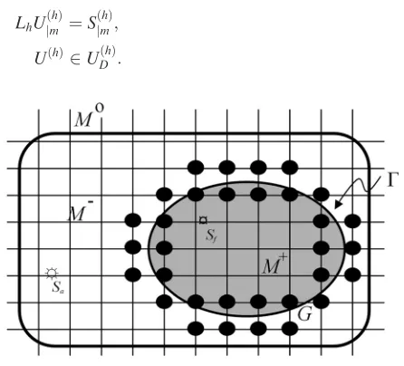
In order to consider the discrete formulation of the ASC problem, some grid in the entire space is introduced. The nodes belonging to the domain to be shielded form set Mþ, while the other nodes represent setM–(see Fig.1). The total combination of the nodes gives us the set M0. The primary acoustic sources can either belong to Mþ or to its exterior

M–. In this formulation, wanted sound sourcesSf are inside

Mþ, while sourcesSasituated outsideM–, are considered as

“unwanted.”

In the discrete formulation of the ASC problem it is required to find such additional sources that the total field from the primary and secondary sources coincides with the wanted sound on grid setMþ.

The boundary value problem (1), (2) is assumed to be approximated by the following:

LhU ðhÞ jm ¼S

ðhÞ jm;

UðhÞ2UDðhÞ: (3)

FIG. 1. Finite difference ASC problem,C: boundary,Mþ: discrete

Suppose that the right-hand side in Eq.(3)consists of wanted and unwanted primary sourcesSðhÞ_f andSðhÞa as well as

con-trolsG(h),

SðhÞ¼SðhÞ_f þSðhÞ_a þGðhÞ:

The general solution to the foregoing finite-difference AS prob-lem can be obtained via the theory of difference potentials

GðhÞ¼ hðMÞLhVðhÞ: (4)

Here,h(M) is the indicator function equal to 1 on the setM

which includes the grid boundary, and equal to 0 anywhere else.

In formula(4),V(h)is an arbitrary function such that

V_CðhÞ¼UðhÞ_C (5)

on the boundary C, where V2UDðhÞ. In practice, the grid

functionUðhÞ_C can be measured.

As shown, e.g., in Ref.14for the ASC solution, it is suffi-cient to have an access only to the trace of the total acoustic field on the boundaryC. In other words, no knowledge of the actual sources (wanted and unwanted) is required. Thus, such active controls are more practical than controls determined by only unwanted field, which may not be separable from the wanted sound. This capability is potentially very useful for applications related to noise control and room acoustics, as it enables protection of the predefined space against the noise coming from the outside, while at the same time not interfer-ing with the ability of the listener to listen to wanted sound from different domains or communicate across the rooms.

To demonstrate the meaning of controls (4), assume that the governing equation in (1) is represented by the Euler acoustics equations with

@p

@t þqc

2_r

u¼qc2qvolþfp;

@u

@t þ

rp

q ¼

bvol

q þfu: (6)

Here, fpand fu are source functions for the continuity and

momentum equations, respectively.

In the continuous space, the counterpart of control (4) is given by (see Refs.21and28)

qvol¼unðCÞdðCÞ;

~

bvol¼~npðCÞdðCÞ: (7)

Here,~nis the external normal to the boundaryCof the pro-tected domain,d(C) is the delta-function assigned to the sur-face C,unis a normal component of particle velocity to C,

p(C) is acoustic pressure. The values of bothun(C) andp(C)

can be obtained from measurements on the boundary, and they normally correspond to the total sound field composed of both the unwanted and wanted components.

Note that if the wanted sound is absent, then the ASC solution will be equivalent to that given by the JMC method.16,29 It appears that the JMC solution applies to a

broader range of conditions than the one under which it was originally derived (see Refs. 15 and30). In particular, it is not limited by unbounded domains without wanted sources. However, if the wanted sound is present then the JMC-based approach cannot be applicable if the controls operate on the basis of the total field from both primary and secondary sources.

Finally, it is worth noting that even though we have ex-plicitly obtained the control sources, their subsequent opti-mization or due allowance for diffraction effects may require the solution of an additional problem (see Ref.31). If the shape of the protected region is complicated, then the unique capability of the DPM to efficiently resolve the geo-metric attributes becomes very important.

III. NUMERICAL SIMULATION

A. Noise shielding

The general solution(7)is applicable in the general case of full 3D flow field in theory. As shown in Ref.31, to obtain the ASC solution based on difference potentials in bounded or unbounded domains, one needs to know only the normal component of the particle velocity at the control boundary of the shielded domain.

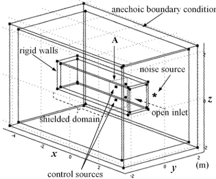
The following simulation case is done in a square duct which is perfectly rigid to allow no energy losses through the duct walls. The duct is 4 m in length and 1 m in width and height for the inner cross-section. The shielded domain is defined to be three times longer in length than the height of the square control surface, so that the measurement can show clearly the effectiveness of the cancellation at positions far away from the control sources. As illustrated in Fig. 2, the noise source is situated outside of the duct at 1 m away from the open inlet of the duct, whereas the shielded domain stretches from the control surface “A” all the way to the left end. The size of the domain is 3 m in length. The noise source is placed off center outside the duct to generate a three-dimensional sound field more effectively. The system can be either with or without a wanted sound. On the control surface four discrete control units each consisting of a dipole and a monopole source, are used.32Theoretically, it has been

shown that at least four control units are required (three per wavelength in each direction) for three-dimensional ASC to achieve a level of 40 dB attenuation on a relatively simple active boundary surface.33

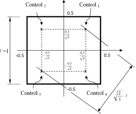
For effective attenuation the distance between sources is recommended to be less thank=2.34That is, the wave length should be longer than twice the diagonal distance of the sources, which translates into

f < c

2L;

here L is a diagonal distance of the sources, i.e., pffiffiffiffiffiffiffiffi2=3 in Fig. 3. Hence, the range for the test frequency should be

f<210 Hz in the simulation. In addition, the size of the dis-crete surface element (effective surface area of each source unit), i.e., 1=4 m2 in Fig. 3, should also be smaller than

k2=4p.33,35 This implies a further condition that f<194 Hz in our particular test case. However, to ensure that a three-dimensional sound field is produced in the simulation, a test frequency of 250 Hz is chosen. This is higher than the cutoff frequency of the (1,1) mode of the square duct, so that the higher order (1,1), (1,0), and (0,1) modes as well as the fun-damental mode will all be excited. The frequency is higher than the upper bound frequency of 194 Hz that was derived from the set-up of the control sources, which means that the effectiveness of the control may be reduced. However, it is more important here to use a higher frequency to demon-strate the three-dimensional applicability of the method. The one-dimensional effectiveness of the method has already been demonstrated in our previous publication.22 The num-ber of control sources is kept to four in the numerical simula-tions as that coincides with the number of controls used in the experiment in Sec.IV.

In practice, to maximize the efficiency of attenuation in 3D space, the optimum distribution of the control sources on boundary surfaces has to be defined. Optimization of the control sources with respect to different criteria has been studied by Loncaric and Tsynkov in Refs. 36 and37. The

distribution of four sets of controls on a square boundary sur-face can be optimized by putting each set at a position deter-mined by the length of each edge times 1=pffiffiffi3in Fig.3.

At each control point on the boundary surface the total sound pressure and particle velocity of the initial sound are measured before calculating the ASC solution. Based on the measurement the ASC solution, (7), defines the strength of control sources which are also situated at the measuring point. When the proposed solution is applied, the result shown in Fig.4(a)and4(b)confirms that it is able to cancel the unwanted noise through the entire shielded domain. In the figure, the sound pressure is shown along the cross-sectionalx-yplane of the duct. The attenuation estimated by the simulation is from 30 to 68 dB when the controls are acti-vated on the control boundary at 250 Hz. In the simulation the propagation of unwanted noise is clearly not unidirec-tional because of the three-dimensional reverberation. The simulation confirms that the method is applicable to such reverberant cases in 3D space.

Figure4(a)and4(b)also shows the important point that the initial sound field does not change outside of the shielded domain, where x>0.8 or x<3 m, while the controls are activated. This particular feature is potentially very useful for real time realization of the control system, since the noise field without the controls can be measured directly outside the shielded domain but in the close neighborhood of the boundary even when the controls are on. Moreover, this shielding method can be seen as a safer method since the sound field remains the same (and not increased by the con-trols) outside the domain while the ASC solution is applied.

The result of the sound pressure distribution on thex-y

plane illustrated in Fig. 4 shows that the whole aimed do-main is shielded when the controls are switched on. This ability of global noise cancellation and preservation of wanted sound based on the method has been theoretically proven in Refs.14and21.

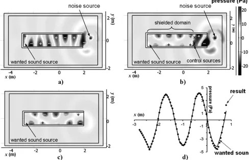
B. Preservation of the wanted sound

To demonstrate the distinct capabilities of the potential-based noise control methodology further, an additional simu-lation is carried out in which a wanted sound source is placed inside the shielded domain. For the study the same configuration of the numerical model illustrated in Fig.2is used except the addition of a wanted sound source situated at the positionx¼ 3,y¼ 0.5,z¼ 0.5 to generate a wanted sound component inside the shielded domain as shown in Fig. 5. Again, we assume that the noise, the wanted sound, and the properties (e.g., reflection properties) of the walls are unknown.

The control sources for ASC are placed on the boundary surface of the protected volume. In order to determine the strength of the control sources, the sound pressure and parti-cle velocity of the total acoustic field (the sum of the adverse noise and wanted sound) are measured at the boundary. Then, the strength of the acoustic monopole and dipole is derived as shown in the above section using Eq.(7). The key point is that there is no need to distinguish between the wanted sound and the noise explicitly in the measurements.

This is possible because the sources of the wanted sound and unwanted sound are on different sides of the boundary of the shielded domain. The measurement of the particle velocity at the boundary is able to capture this information inherently. When the control devices are applied, the dipole source pro-vides the necessary directional element that allows the can-cellation of sound from outside the shielded domain (the unwanted sound) but not from the inside (the wanted sound). Figure 5illustrates the general configuration of the simula-tion model on thex-yplane with sound pressure distribution when the controls are turned off.

Figure 6 illustrates the sound pressure distribution, at 250 Hz, in the case described above in Fig. 5. The light and shade in Fig. 6(a) show the initial sound pressure when the noise and wanted sounds are both switched on, while the con-trol sources are still off. Figure6(b)represents the net sound pressure field when the noise is canceled out after the activa-tion of the AS control sources. For comparison, the original wanted sound is separately measured at the same reference position when both the AS control and unwanted noise sour-ces have been turned off. This is shown in Fig.6(c). The result upon shielding and the original wanted sound along x axis (y¼0) in the shielded domain are overlaid in Fig.6(d)to give a clearer view. Obviously, when the unwanted noise becomes stronger relative to the wanted sound, the error between them increases due to the decrease in signal to noise ratio.

However, even at a signal to noise ratio of10 dB, the ampli-tude error has been reported to be theoretically less than 1 dB in the authors’ previous study on one-dimensional AS prob-lems.22 Fig. 6(d) shows the similarity between the original wanted sound pressure—and the result • when the controls are switched on. In the simulation, a challenging condition is set up by introducing a significantly bigger unwanted sound pres-sure than the wanted one (about 10 dB higher), so that the results can give a reliable guidance of the attenuation that can be achieved in practice when the wanted sound has been seri-ously contaminated by strong unwanted noise. Figure 6(d)

also shows that, on the whole, the total sound field with the potential-based control sources resembles closely the original wanted sound field at each measuring position everywhere in the shielded domain.

The similarity between the net sound field shielded by the AS control sources and the original wanted sound field is also evaluated by the cross-correlation of the two results. When the AS control sources are switched on, the cross-correlation of the wanted sound and the shielded total sound pressure (unwanted noise, wanted sound, and sound field with the controls) is 0.998. The ideal cross-correlation of two identical signals is 1.0. This is almost achieved in the simulation, which shows that the shielded net sound field with the controls on matches the original wanted sound field very well. The numerical simulation clearly proves that wanted sound can be very effectively protected by the active controls based on the proposed method even in a three-dimensional problem where both wanted sound and unwanted noise are unknown, while noise is significantly suppressed by the AS control sources.

IV. EXPERIMENT

The performance of the active shielding technique in three-dimensional is tested in an experiment. The solution for the ASC problems either with or without the wanted sounds has previously been experimentally validated in a one-dimensional duct, and the results were reported in Refs.

22 and25. Following those works, this experiment extends the methodology to a three-dimensional problem. In the experiment we concentrate our effort in a case without

FIG. 4. Sound pressure distribution (a) of noise and (b) of the sum of noise and control output at 250 Hz onx-yplane, where4<x<3,2<y<2,z¼0 in

3D space.

FIG. 5. Configuration with unwanted and wanted sound sources in a 3D

wanted sound in a dimensional space. For the three-dimensional case, two-three-dimensional arrays of actuators and microphones are required on the boundary surfaces to realize the shielding of a given volume. The key factors investigated in this realization of the three-dimensional ASC are the physical size, number, and positioning of the control sources (actuators) and monitoring microphones. In the experiment they are optimized in order to achieve the best noise cancel-lation in the shielded domain. The experimental model stated in this section is accurately designed and tested. It is based on the difference potential theory which is studied in Sec.

III. For example, source positions, measuring method, and the number of controls are strictly defined using the original theory.

The sound generation system consists of loudspeakers, power amplifiers, digital signal processing (DSP) modules, and a PC with multi-channel sound cards. The audio data measured on the active surfaces are fed into the control sys-tem through an Alesis Digital Audio Tape Protocol (ADAT) converter first. The converted data are sent to a Multi-channel Audio Digital Interface (MADI) converter. After all these conversions, the resulting data are stored in a computer through MADI card and can be used for further DSP manip-ulation. The data received in the computer are then incorpo-rated into the ASC algorithm together with the calibincorpo-rated loudspeaker transfer functions and directivity to generate the desired sound signals, which are then saved as

phase-synchronous audio data files, which can be played back using a multi-channel audio editor. In the system, after the filtering process the signals are led to the ADAT matrix which splits them to provide each input channel of a render with an output signal. After played back by the render, the separate audio signals are converted to MADI and sent to the MADI-ADAT converter via RME HDSP sound cards with 64 channel outputs in MADI format and then ADAT-audio converter successively.

To estimate the actual accuracy of the control system in the experiment, the phase error in degrees between the input signal and the DSP apparatus is determined through a set of preliminary measurements. Figures 7(a) and 7(b)

show such an error measured over a range of frequencies up to 1.5 kHz with swept sine excitation. The results shown in Fig.7(a)demonstrate experimentally that the error in the control system at the frequencies chosen for the test, i.e., above 90 Hz, is largely below 0.15 degrees in phase. Therefore, according to the theoretical sensitivity analysis reported in the earlier publication Ref. 23, an AS system with these errors should allow us to achieve about 50–55 dB attenuation.25 This is indeed consistent with the attenuation we obtained in the numerical analysis. The cor-responding time delay error, which can be caused by the DSP apparatus, is below 8lsec. if the frequency is above 60 Hz in Fig. 7(b). This has been measured at a sampling frequency of 44.1 kHz.

FIG. 6. Sound pressure distribution in a space, where4<x<3,2<y<2,z¼0 at 250 Hz: (a) the sound pressure of noise and wanted sound without

con-trol, (b) shielded total sound pressure (the sum of noise, wanted sound and control output), (c) wanted sound pressure, and (d)—: wanted sound pressure, and

The sound generating system consists of loudspeaker arrays and power amplifiers. A driver is chosen to guarantee good stiffness, dynamic stability, and low distortion degree. The driver shows a quite stable linear frequency response especially in the test frequency range, i.e., below 500 Hz. The sensitivity errors of each driver are about 1 dB in the range between 90 and 250 Hz and about 3 dB between 80 and 1500 Hz. A3 dB cut-off frequency and the resonance frequency appear at 80 Hz. The sensitivity of a driver is 82 dB at 2.83 v/1 m. The effective piston area of the driver is 0.003 m2. Each set of the control is designed with a dipole and monopole source. In addition, a loudspeaker is also used as an external noise source. Each secondary source set is constructed with thick medium-density fiber-board (MDF) enclosures and clamped directly on the supporting metal bar.

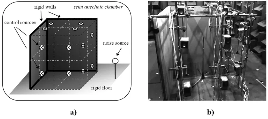
A shielded domain is defined in a cube with 1.5 m in each side length. The three sides of the domain are terminated by two rigid walls and a floor. The other sides are acoustically transparent and allow propagation of three-dimensional sound fields through them. The cube sits on the floor of a semi-anechoic chamber. In this setup the effect of reflection on the walls does not need to be considered separately as it is consid-ered automatically.14,31This capability belongs to the original

nature of the method. Therefore, we believe that the method is practically applicable in a wide range of applications even with randomly incoming reflected sound.

To make the experimental model more general, and to take advantage of the potential-based method’s ability to work without precise knowledge of system conditions, the acoustic properties of the walls and floor are not known in the experi-ment, and are not needed in the potential-based approach. To generalize the experiment further, the position of the noise source is supposed to be unknown. The noise is generated by a broadband white noise signal containing an equal amount of all frequencies in the range between 50 and 250 Hz. Figure

8(a)illustrates the positions of an unwanted noise source out-side of the domain and control sources on the boundary surfa-ces. Figure 8(b) shows the general configuration of a two-dimensional active boundary surface consisting 12 control sets arranged at the control points in the realization.

The direction of the dipole source mounted on the bound-ary defines the inside and outside of a shielded domain. For this reason the direction of the dipole source must be perpen-dicular to the boundary and pointed out from the shielded do-main. The sound pressure and particle velocity are measured on the perimeter of each control source set. The distribution of four sets of controls on a square boundary surface can be

FIG. 8. Experimental setup.

optimized by putting each set at a position determined by the length of each edge times 1=pffiffiffi3(see Fig. 3). The measured values, adjusted for the transfer-function of the signal genera-tor, are used to calculate offline the control source signals based on the difference potential theory.

In the measuring process, before obtaining the ASC sol-utions for a given problem, directional and non-directional components of the sound field are measured using a B&K PULSE Sound & Vibration analyzer with the control sources off. The former is the normal component of the particle ve-locityuo, and the latter is the acoustic pressurepoof the total

field at the boundary. Then, the directional component meas-ured defines a non-directional control source which is a monopole. The non-directional component measured is used to define a dipole control source which is directional.

The source strengths of the controlsbandqnormalized to the reference signalVref are

^

b¼p^oAs

Hd

; q^¼ðu^o~nÞAs

Hm

: (8)

Hereb^¼b/Vref,q^¼q/Vref,p^o¼po/Vref, andu^o¼uo/Vref.As

is a surface area element, Hd is the transfer-function of the

dipole source signal generator, Hm is the transfer-function of

the monopole source signal generator, and~n is a unit normal vector on the boundary surface in Eq. (7). Then, the control source signals are saved as phase-synchronous.wav files which can be played back using a multi-channel signal generator.

A typical example of the ASC results based on difference potentials in a three-dimensional space is shown in Fig.9. To test the capability of the method in practical cases, a white noise source is used in a room to generate a three-dimensional sound filed in the experiment.

The listening position is located at the middle of the shielded domain surrounded by the three active surfaces and three hard walls. The distance between each control source on a surface is 2/31.5 m. The frequency range is limited to below 250 Hz in the experiment due to this distance between control sources on each side of the cube.

The rigid line in Fig. 9shows the initial sound pressure distribution when the noise is activated, while the control sour-ces are still off. The dotted line represents the distribution of the net sound pressure when the noise is suppressed by the con-trols. When the control sources are activated, the control sys-tem attains attenuations of around 5 to 13 dB in the middle of the shielded domains at the frequency range of 80 to 220 Hz.

Because of the difficulty in dealing with a number of bulky control sources and the complexity of three dimen-sional sound fields, the result in this section shows lower ef-ficiency in the overall attenuation, when compared with the result achieved in a one-dimensional experiment and reported in the previous publication, which was around 15 to 20 dB.22One of the main reasons can be found in the design of the experimental model. That is, the control sources them-selves cause disturbances to the sound fields. These distur-bances near the active boundary surface were not considered in the design of this experimental model.

Near 150 Hz, the control sources are about multiples of a 3/4 wavelength from the hard surfaces where the sound

pressure is low. As a result, the output of the controls becomes very small and noise shielding is not effective near this particular frequency (see Fig.9).

The experiment demonstrates that the potential-based ASC automatically extracts all the necessary information about the system and the unwanted noise itself from the measurements performed at the boundary surface. The experiment proves the potential possibilities of suppression of unwanted noise by the active controls based on the proposed method even in a three-dimensional space, although significant challenges remain in how to account for the presence of the control sources.

V. CONTROL OUTPUTS

The proposed approach in this paper can be realized pro-vided that the contribution of the control sources to the input data can be separated. A natural question to follow up is if the solution can still be obtained without such separation in practice. Two simulated cases are examined to answer this.

Figure10shows the case when there is no wanted sound. The result shows that the contribution of the controls vanishes everywhere outside the domain in Fig.10(b). The key factor is the direction of the dipole source defining the inside or outside of a domain. The output of the dipole source at the control point exactly cancels any monopole source contribution out-side the shielded domain. However, inout-side the domain the sign of the dipole source is reversed, and the combination of the dipole source and monopole source produces the sound field that is 180 degrees out of phase with the noise and cancels the noise inside the domain [compare Figs.10(a)and10(b)].

Therefore, the contribution of the dipole and monopole sources based on solution (7)in the absence of any wanted sound is summarized as follows:

pmþpdðqÞ ¼ pa;inside shielded domain

and

pmþpdðqþÞ ¼0;outside the domain:

Herepais the pressure of adverse noise.

In cases where there is no wanted sound to be preserved, as in Fig.10(b), the simulation result shows that the controls do not make any additional sound field anywhere outside of the shielded domain. Hence in this case, it could be possible to measure the sound field without the controls near the out-side boundary of the shielded domain even when the controls are on.

In a further simulation, wanted sound pressure with magnitude twice that of the unwanted noise is introduced into the space, so that the output of the controls can be

investigated to show its relationship with either the wanted sound, noise or none of them in each domain (inside, or out-side the shielded domain). In the shielded domain the same conclusion of Fig. 10is applicable to the case with wanted sound, as illustrated in Fig.11. The plots shown in Fig. 11

are brought from the result described in Sec.III B. Figure11

shows that the output of the controls produces the sound field 180 degrees out of phase with the noise inside the domain ei-ther with or without a wanted sound. However outside shielded domain, unlike the conclusion of the case without a

FIG. 11. Plots of sound pressure distribution alongxaxis in a 3D space. Sound pressure of x: noise,- -: wanted sound, and䉫: control output without noise

and wanted sound at 250 Hz.

wanted sound, the output of the controls now duplicates the wanted sound field. It makes the sound outside the shielded domain to be 6 dB louder after the controls are switched on. Hence, even in the case with wanted sound, it may still be feasible to deduce the sound field without contribution from the controls by having the value of the measured sound field near the outside boundary of the shielded domain when the controls are on.

The results above show that it may be possible to deter-mine the original sound field without switching off the con-trol sources, which could then lead to a real time realization of a practical adaptive active shielding methodology. A proper mathematical framework for this will be developed in a further work.

VI. CONCLUSIONS

The practicality of active shielding based on the method of difference potentials has been demonstrated and validated with broadband acoustic sources in a three-dimensional space. It has been shown that attenuation of around 12 dB has been achieved in the experiment in a large volume of a shielded domain. Apart from the practical difficulties associ-ated with the realization of control source arrays on the boundary surface, the results of the experiment and numeri-cal analysis show that the method can provide an effective solution in a three-dimensional space through a broadband spectrum of low frequencies.

The physical size of the control sources has been considered as one of the reasons that limit the performance of the system. This is a common problem in most existing active control meth-ods. The size of a control source is still a factor restricting the effective frequency range for suppression of noise. In addition to the suppression of noise, the proposed method has been shown through numerical simulations to effectively preserve the wanted sound separately from the total fields composed of noise and wanted sound, in three-dimensional spaces where the sys-tem characteristics are not known. The results clearly demon-strate the potential advantages of the method under these extended experimental conditions. All the current set of experi-ments has been limited to a non-real-time control system. The proposed approach has only been tested in experiments where the contribution of the control sources can be completely sepa-rated. However, the numerical simulation and theoretical studies have shown that, in cases where there is no wanted sound, the proposed approach in its present form can be applicable in real-time system since the noise field without the control outputs can be measured directly in the close neighborhood of the boundary. In cases with wanted sound, additional on-line calculations will be required for the separation of control outputs from input data. Future research will focus on the development and study of the real-time active control, and on the extension of the method to the case with three-dimensional wanted sound field.

ACKNOWLEDGMENTS

The research was supported by the Engineering and Physical Sciences Research Council (EPSRC) under the project codes, GR/T26825 and GR/T26832/01.

NOMENCLATURE

bvol Force per unit volume

c Speed of sound

L Operator

qvol Volume velocity per unit volume

t Time

u Particle velocity

q Air density

SUBSCRIPTS

a Adverse sound (noise)

d Dipole

m Monopole

jm Value at nodem D Value in a domainD

h Discrete counterpart

SUPERSCRIPTS

(h) _{Discrete function}

1_{R. K. Kincaid, S. L. Padula, and D. L. Palumbo, “Optimal sensor/actuator}

locations for active structural acoustic control,” AIAA Paper 98-1865, in Proceedings of the 39th AIAA/ASME/ASCE/AHS/ASC Structures, DynamicsandMaterialsConference (Long Beach, CA, 1998).

2_{R. K. Kincaid and K. Laba, “Reactive tabu search and sensor selection in}

active structural control problems,” J. Heuristics4, 199–220 (1998).

3

J. Piraux and B. Nayroles, “A theoretical model for active noise

attenua-tion in three-dimensional space,” inProceedings of Internoise’80, Miami

(1980), pp. 703–706.

4

P. A. Nelson, A. R. D. Curtis, S. J. Elliott, and A. J. Bullmore, “The mini-mum power output of free field point sources and the active control of

sound,” J. Sound Vib.116, 397–414 (1987).

5_{T. Kletschkowski, “Adaptive feed-forward control of low frequency}

inte-rior noise,” inIntelligent Systems, Control and Automation: Science and

Engineering(Springer, New York, 2012), 330 p.

6_{K. Kochan, D. Sachau, and H. Breitbach, “Robust active noise control in}

the loadmaster area of a military transport aircraft,” J. Acoust. Soc. Am.

129(5), 3011–3019 (2011).

7

S. Bohme, D. Sachau, and H. Breitbach, “Optimization of actuator and

sensor positions for an active noise reduction system,” inProceedings of

SPIE 6171(San Diego, CA, 2006).

8

C. D. Petersen, R. Froonje, B. S. Cazzolato, A. C. Zander, and C. H. Hansen, “A Kalman filter approach to virtual sensing for active noise

con-trol,” Mech. Syst. Signal Process.22, 490–508 (2008).

9_{N. Epain and E. Friot, “Active control of sound inside a sphere via control}

of the acoustic pressure at the boundary surface,” J. Sound Vib. 299,

587–604 (2007).

10_{B. Kwon and Y. Park, “Active window based on the prediction of interior}

sound field: Experiment for a band-limited noise,” in Proceeding of Inter-Noise 2011, Osaka, Japan (2011), Vol. 4, pp. 443–446.

11

G. D. Malyuzhinets, “An unsteady diffraction problem for the wave equa-tion with compactly supported right-hand side (in Russian),” in Proceedings of the Acoustics Institute (USSR Academy of Science, Moscow, Russia, 1971), pp. 124–139.

12

S. V. Tsynkov, “On the definition of surface potentials for

finite-difference operators,” J. Sci. Comput.18, 155–189 (2003).

13_{V. S. Ryaben’kii, “A difference shielding problem,” J. Funct. Anal. Appl.}

29(1), 70–71 (1995).

14

V. S. Ryaben’kii,Method of Difference Potentials and its Applications

(Springer-Verlag, Berlin, 2002), pp. 515–522.

15_{M. J. M. Jessel and G. A. Mangiante, “Active sound absorbers in an air}

duct,” J. Sound Vib.23(3), 383–390 (1972).

16

G. A. Mangiante, “Active sound absorption,” J. Acoust. Soc. Am.61(6),

1519–1522 (1977).

17_{G. Canevet, “Active sound absorption in air conditioning duct,” J. Sound}

18

J. C. Burgess, “Active adaptive sound control in a duct: A computer

simu-lation,” J. Acoust. Soc. Am.70, 715–726 (1981).

19

S. J. Elliot, P. A. Nelson, and I. M. Stothers, “A multiple error LMS algo-rithm and its application to the active control of sound and vibration,”

IEEE Trans. Acoust. Speech Signal Process.35, 1423–1434 (1987).

20

S. E. Wright and B. Vuksanovic, “Active control of environment noise II:

Non-compact acoustic sources,” J. Sound Vib.202, 313–359 (1997).

21_{V. S. Ryaben’kii, S. V. Utyuzhnikov, and A. Turan, “On the application of}

difference potential theory to active noise control,” J. Adv. Appl. Math.

40(2), 194–211 (2008).

22

H. Lim, S. V. Utyuzhnikov, Y. W. Lam, and A. Turan, “Multi-domain

active sound control and noise shielding,” J. Acoust. Soc. Am. 129(2),

717–725 (2011).

23

S. V. Utyuzhnikov, “Nonstationary problem of active sound control in

bounded domains,” J. Comput. Appl. Math.234(6), 1725–1731 (2010).

24_{H. Lim, Y. W. Lam, and S. V. Utyuzhnikov, “Active control system for}

global cancellation of noise while preserving wanted sound in multi-domains,” in Proceedings of Inter-Noise 2011, Osaka, Japan (2011), Vol. 6, pp. 419–424.

25_{H. Lim, S. V. Utyuzhnikov, Y. W. Lam, A. Turan, M. R. Avis, V. S.}

Ryaben’kii, and S. V. Tsynkov, “Experimental validation of the active

noise control methodology based on difference potentials,” AIAA J.47(4),

874–884 (2009).

26_{H. Lim, “Active shielding based on difference potentials,” Ph.D. thesis,}

The University of Salford, Salford, UK, 2011, 198 p.

27

J. Loncaric, V. S. Ryaben’kii, and S. V. Tsynkov, “Active shielding and

control of noise,” SIAM J.62(2), 563–596 (2001).

28

S. V. Utyuzhnikov, “Active wave control and generalized surface

potentials,” J. Adv. Appl. Math.43(2), 101–112 (2009).

29_{S. Uosukainen, “Modified JMC method in active control of sound,” Acust.}

Acta Acust.83, 105–112 (1997).

30

P. Lueg, “Process of silencing sound oscillations,” U.S. patent No. 2043416 (1936).

31_{V. S. Ryaben’kii and S. V. Utyuzhnikov, “Active shielding model for}

hyperbolic equations,” IMA J. Appl. Math.71(6), 924–939 (2006).

32

V. S. Ryaben’kii, S. V. Tsynkov, and S. V. Utyuzhnikov, “Active control of sound with variable degree of cancellation,” J. Appl. Math. Lett.

22(12), 1846–1851 (2009).

33

P. A. Nelson and S. J. Elliott,Active Control of Sound(Academic Press,

San Diego, CA, 1992), pp. 116–122, 143–146, 311–378.

34_{P. Berglund, “Investigation of acoustic source characterisation and}

instal-lation effects for small axial fans,” TRITA-FKT Rep. 2003:02, Royal Institute of Technology, Stockholm, Sweden, (2003), p. 44.

35

O. Tochi and S. Veres,Active Sound and Vibration Control: Theory and

Applications(The Institution of Engineers, London, 2002), p. 6.

36_{J. Loncaric and S. V. Tsynkov, “Optimization of acoustic source strength}

in the problems of active noise control,” SIAM J. Appl. Math. 63,

1141–1183 (2003).

37_{J. Loncaric and S. V. Tsynkov, “Optimization of power in the problem of}