Models for Heavy-tailed Asset Returns
Borak, Szymon and Misiorek, Adam and Weron, Rafal
Wrocław University of Technology, Poland
September 2010
Online at
https://mpra.ub.uni-muenchen.de/25494/
Models for Heavy-tailed
Asset Returns
1
Szymon Borak
2, Adam Misiorek
3, and
Rafał
Weron
4Abstract: Many of the concepts in theoretical and empirical finance developed
over the past decades
–
including the classical portfolio theory, the
Black-Scholes-Merton option pricing model or the RiskMetrics variance-covariance
approach to VaR
–
rest upon the assumption that asset returns follow a normal
distribution. But this assumption is not justified by empirical data! Rather, the
empirical observations exhibit excess kurtosis, more colloquially known as fat
tails or heavy tails. This chapter is intended as a guide to heavy-tailed models.
We first describe the historically oldest heavy-tailed model
–
the stable laws.
Next, we briefly characterize their recent lighter-tailed generalizations, the
so-called truncated and tempered stable distributions. Then we study the class of
generalized hyperbolic laws, which
–
like tempered stable distributions
–
can be
classified somewhere between infinite variance stable laws and the Gaussian
distribution. Finally, we provide numerical examples.
Keywords: Heavy-tailed distribution; Stable distribution; Tempered stable
distribution; Generalized hyperbolic distribution; Asset return; Random number
generation; Parameter estimation
JEL: C13, C15, C16, G32
1
Chapter prepared for the 2
ndedition of
Statistical Tools for Finance and Insurance
, P.Cizek,
W.Härdle, R.Weron (eds.), Springer
-Verlag,
forthcoming
in 2011
.
2
Deutsche Bank AG, London, U.K.
3
Santander Consumer Bank S.A., Wrocław, Poland
Returns
Szymon Borak, Adam Misiorek, and Rafa l Weron
1.1
Introduction
Many of the concepts in theoretical and empirical finance developed over the past decades – including the classical portfolio theory, the Black-Scholes-Merton option pricing model or the RiskMetrics variance-covariance approach to Value at Risk (VaR) – rest upon the assumption that asset returns follow a normal distribution. But this assumption is not justified by empirical data! Rather, the empirical observations exhibit excess kurtosis, more colloquially known as
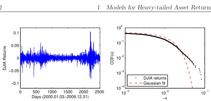
fat tailsorheavy tails (Guillaume et al., 1997; Rachev and Mittnik, 2000). The contrast with the Gaussian law can be striking, as in Figure 1.1 where we il-lustrate this phenomenon using a ten-year history of the Dow Jones Industrial Average (DJIA) index.
In the context of VaR calculations, the problem of the underestimation of risk by the Gaussian distribution has been dealt with by the regulators in anad hoc way. The Basle Committee on Banking Supervision (1995) suggested that for the purpose of determining minimum capital reserves financial institutions use a 10-day VaR at the 99% confidence level multiplied by a safety factor
s∈[3,4]. Stahl (1997) and Danielsson, Hartmann and De Vries (1998) argue convincingly that the range ofsis a result of the heavy-tailed nature of asset returns. Namely, if we assume that the distribution is symmetric and has finite varianceσ2 then from Chebyshev’s inequality we have P(Loss≥ǫ)≤ 1
2σ
2ǫ2.
Setting the right hand side to 1% yields an upper bound for VaR99%≤7.07σ.
On the other hand, if we assume that returns are normally distributed we arrive at VaR99%≤2.33σ, which is roughly three times lower than the bound
0 500 1000 1500 2000 2500 −0.1
−0.05 0 0.05 0.1
Days (2000.01.03−2009.12.31)
DJIA Returns
10−3 10−2 10−1 10−4
10−3 10−2 10−1 100
−x
CDF(x)
[image:4.595.172.508.107.269.2]DJIA returns Gaussian fit
Figure 1.1:Left panel: Returns log(Xt+1/Xt) of the DJIA daily closing values
Xt from the period January 3, 2000 – December 31, 2009. Right
panel: Gaussian fit to the empirical cumulative distribution func-tion (cdf) of the returns on a double logarithmic scale (only the left tail fit is displayed).
STF2stab01.m
Being aware of the underestimation of risk by the Gaussian law we should consider using heavy-tailed alternatives. This chapter is intended as a guide to such models. In Section 1.2 we describe the historically oldest heavy-tailed model – the stable laws. Next, in Section 1.3 we briefly characterize their re-cent lighter-tailed generalizations, the so-called truncated and tempered stable distributions. In Section 1.4 we study the class of generalized hyperbolic laws, which – like tempered stable distributions – can be classified somewhere be-tween infinite variance stable laws and the Gaussian distribution. Finally, in Section 1.5 we provide numerical examples.
1.2
Stable Distributions
1.2.1
Definitions and Basic Properties
(asymp-−10 −5 0 5 10 10−4
10−3 10−2 10−1
x
PDF(x)
−50 −2.5 0 2.5 5 0.05
0.1 0.15
x
PDF(x)
α=2
α=1.9
α=1.5
α=0.5
β=0
β=−1
β=0.5
[image:5.595.87.424.135.269.2]β=1
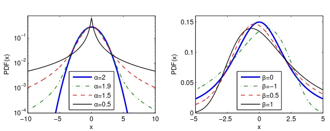
Figure 1.2:Left panel: A semi-logarithmic plot of symmetric (β = µ = 0) stable densities for four values ofα. Note, the distinct behavior of the Gaussian (α= 2) distribution. Right panel: A plot of stable densities forα= 1.2 and four values ofβ.
STF2stab02.m
totically) normally distributed. Yet, this beautiful theoretical result has been notoriously contradicted by empirical findings. Possible reasons for the fail-ure of the CLT in financial markets are (i) infinite-variance distributions of the variables, (ii) non-identical distributions of the variables, (iii) dependences between the variables or (iv) any combination of the three. If only the finite variance assumption is released we have a straightforward solution by virtue of the generalized CLT, which states that the limiting distribution of sums of such variables is stable (Nolan, 2010). This, together with the fact that stable distributions are leptokurtic and can accommodate fat tails and asymmetry, has led to their use as an alternative model for asset returns since the 1960s.
the right tail is thicker, see the right panel in Figure 1.2. When it is negative, it is skewed to the left. When β = 0, the distribution is symmetric about the mode (the peak) of the distribution. Asαapproaches 2,β loses its effect and the distribution approaches the Gaussian distribution regardless ofβ. The last two parameters,σ >0 andµ∈R, are the usual scale and location parameters, respectively.
A far-reaching feature of the stable distribution is the fact that its probability density function (pdf) and cumulative distribution function (cdf) do not have closed form expressions, with the exception of three special cases. The best known of these is the Gaussian (α= 2) law whose pdf is given by:
fG(x) = √1
2πσexp
−(x−µ)
2
2σ2
. (1.1)
The other two are the lesser known Cauchy (α= 1,β = 0) and L´evy (α= 0.5,
β = 1) laws. Consequently, the stable distribution can be most conveniently described by its characteristic function (cf) – the inverse Fourier transform of the pdf. The most popular parameterization of the characteristic functionφ(t) ofX ∼Sα(σ, β, µ), i.e. a stable random variable with parametersα,σ, β and
µ, is given by (Samorodnitsky and Taqqu, 1994; Weron, 1996):
logφ(t) =
−σα|t|α{1−iβsign(t) tanπα
2 }+iµt, α6= 1,
−σ|t|{1 +iβsign(t)π2log|t|}+iµt, α= 1.
(1.2)
Note, that the traditional scale parameterσof the Gaussian distribution is not the same asσin the above representation. A comparison of formulas (1.1) and (1.2) yields the relation: σGaussian=
√
2σ.
For numerical purposes, it is often useful to use Nolan’s (1997) parameteriza-tion:
logφ0(t) =
−σα|t|α{1 +iβsign(t) tanπα
2 [(σ|t|)
1−α−1]}+iµ
0t, α6= 1,
−σ|t|{1 +iβsign(t)2
πlog(σ|t|)}+iµ0t, α= 1, (1.3) which yields a cf (and hence the pdf and cdf) jointly continuous in all four parameters. The location parameters of the two representations (S and S0)
The ‘fatness’ of the tails of a stable distribution can be derived from the fol-lowing property: the pth moment of a stable random variable is finite if and only ifp < α. Hence, whenα > 1 the mean of the distribution exists (and is equal to µ). On the other hand, when α <2 the variance is infinite and the tails exhibit a power-law behavior (i.e. they are asymptotically equivalent to a Pareto law). More precisely, using a CLT type argument it can be shown that (Janicki and Weron, 1994a; Samorodnitsky and Taqqu, 1994):
(
limx→∞xαP(X > x) =Cα(1 +β)σα,
limx→∞xαP(X <−x) =Cα(1 +β)σα,
(1.4)
where Cα = 2R0∞x−αsin(x)dx
−1
= π1Γ(α) sinπα2 . The convergence to the power-law tail varies for differentα’s and is slower for larger values of the tail index. Moreover, the tails of stable cdfs exhibit a crossover from an approximate power decay with exponent α > 2 to the true tail with exponent α. This phenomenon is more visible for largeα’s (Weron, 2001).
1.2.2
Computation of Stable Density and Distribution
Functions
The lack of closed form formulas for most stable densities and distribution functions has far-reaching consequences. Numerical approximation or direct numerical integration have to be used instead of analytical formulas, leading to a drastic increase in computational time and loss of accuracy. Despite a few early attempts in the 1970s, efficient and general techniques have not been developed until late 1990s.
Mittnik, Doganoglu and Chenyao (1999) exploited the pdf–cf relationship and applied the fast Fourier transform (FFT). However, for data points falling between the equally spaced FFT grid nodes an interpolation technique has to be used. The authors suggested that linear interpolation suffices in most practical applications, see also Rachev and Mittnik (2000). Taking a larger number of grid points increases accuracy, however, at the expense of higher computational burden. Setting the number of grid points toN = 213 and the
Chenyao (1999) report that for N = 213 the FFT based method is faster
for samples exceeding 100 observations and slower for smaller data sets. We must stress, however, that the FFT based approach is not as universal as the direct integration method – it is efficient only for large alpha’s and only as far as the pdf calculations are concerned. When computing the cdf the former method must numerically integrate the density, whereas the latter takes the same amount of time in both cases.
The direct integration method, proposed by Nolan (1997, 1999), consists of a numerical integration of Zolotarev’s (1986) formulas for the density or the distribution function. Set ζ = −βtanπα
2 . Then the density f(x;α, β) of a
standard stable random variable in representation S0, i.e. X ∼ S0
α(1, β,0), can be expressed as (note, that Zolotarev (1986, Section 2.2) used another parametrization):
• whenα6= 1 andx6=ζ:
f(x;α, β) =α(x−ζ)
1
α−1
π|α−1|
Z π2
−θ0
V(θ;α, β) exp
−(x−ζ)α−α1V(θ;α, β) dθ, (1.5) forx > ζ and f(x;α, β) =f(−x;α,−β) forx < ζ,
• when α6= 1 andx=ζ:
f(x;α, β) = Γ(1 +
1
α) cos(ξ)
π(1 +ζ2)1 2α
,
• whenα= 1:
f(x; 1, β) =
1
2|β|e
πx
2β R π
2
−π
2
V(θ; 1, β) expn−eπx2βV(θ; 1, β)
o
dθ, β6= 0,
1
π(1+x2), β= 0,
where
ξ=
(1
αarctan(−ζ), α6= 1, π
2, α= 1,
(1.6)
and
V(θ;α, β) =
(cosαξ)α−11
cosθ
sinα(ξ+θ)
αα−1 cos{αξ+(α−1)θ}
cosθ , α6= 1,
2
π
π
2+βθ
cosθ
The distributionF(x;α, β) of a standard stable random variable in represen-tationS0can be expressed as:
• whenα6= 1 andx6=ζ:
F(x;α, β) =c1(α, β) +
sign(1−α)
π
Z π2
−ξ
exp
−(x−ζ)αα−1V(θ;α, β) dθ,
forx > ζ andF(x;α, β) = 1−F(−x;α,−β) forx < ζ, where
c1(α, β) = (1
π π
2 −ξ
, α <1,
1, α >1,
• whenα6= 1 andx=ζ:
F(x;α, β) = 1
π
π
2 −ξ
,
• whenα= 1:
F(x; 1, β) =
1 π
Rπ2
−π
2 exp
n
−e−πx2βV(θ; 1, β)
o
dθ, β >0,
1
2+
1
πarctanx, β= 0,
1−F(x,1,−β), β <0.
Formula (1.5) requires numerical integration of the function g(·) exp{−g(·)}, whereg(θ;x, α, β) = (x−ζ)αα−1V(θ;α, β). The integrand is 0 at−ξ, increases monotonically to a maximum of 1
e at point θ
∗ for which g(θ∗;x, α, β) = 1,
and then decreases monotonically to 0 at π
2 (Nolan, 1997). However, in some
cases the integrand becomes very peaked and numerical algorithms can miss the spike and underestimate the integral. To avoid this problem we need to find the argumentθ∗ of the peak numerically and compute the integral as a
sum of two integrals: one from−ξtoθ∗ and the other fromθ∗ to π
2.
probably the most efficient (downloadable from John Nolan’s web page: aca-demic2.american.edu/˜jpnolan/stable/stable.html). It was written in Fortran and calls several external IMSL routines, see Nolan (1997) for details. Apart from speed, the STABLE program also exhibits high relative accuracy (ca. 10−13; for default tolerance settings) for extreme tail events and 10−10 for
values used in typical financial applications (like approximating asset return distributions). The STABLE program is also available in library form through Robust Analysis Inc. (www.robustanalysis.com). This library provides inter-faces to Matlab, S-plus/R and Mathematica.
In the late 1990s Diethelm W¨urtz has initiated the development of Rmetrics, an open source collection of S-plus/R software packages for computational finance (www.rmetrics.org). In the fBasics package stable pdf and cdf calculations are performed using the direct integration method, with the integrals being computed by R’s function integrate. On the other hand, the FFT based ap-proach is utilized in Cognity, a commercial risk management platform that offers derivatives pricing and portfolio optimization based on the assumption of stably distributed returns (www.finanalytica.com). The FFT implementa-tion is also available in Matlab (stablepdf fft.m) from the Statistical Software Components repository (ideas.repec.org/c/boc/bocode/m429004.html).
1.2.3
Simulation of Stable Variables
Simulating sequences of stable random variables is not straightforward, since there are no analytic expressions for the inverseF−1(x) nor the cdf F(x)
it-self. All standard approaches like the rejection or the inversion methods would require tedious computations. A much more elegant and efficient solution was proposed by Chambers, Mallows and Stuck (1976). They noticed that a certain integral formula derived by Zolotarev (1964) led to the following algorithm:
• generate a random variable U uniformly distributed on (−π2,
π
2) and an
independent exponential random variableW with mean 1;
• forα6= 1 compute:
X = (1 +ζ2)1
2αsin{α(U +ξ)}
{cos(U)}1/α
cos
{U−α(U+ξ)}
W
1−α α
• forα= 1 compute:
X= 1
ξ
π
2 +βU
tanU−βlog
π
2WcosU
π
2 +βU
, (1.8)
whereξ is given by eqn. (1.6). This algorithm yields a random variableX ∼
Sα(1, β,0), in representation (1.2). For a detailed proof see Weron (1996). Given the formulas for simulation of a standard stable random variable, we can easily simulate a stable random variable for all admissible values of the parametersα,σ,β andµusing the following property. IfX ∼Sα(1, β,0) then
Y =
(
σX+µ, α6= 1, σX+ 2
πβσlogσ+µ, α= 1,
(1.9)
isSα(σ, β, µ). It is interesting to note that forα= 2 (andβ= 0) the Chambers-Mallows-Stuck (CMS) method reduces to the well known Box-Muller algorithm for generating Gaussian random variables.
Many other approaches have been proposed in the literature, including appli-cation of Bergstr¨om and LePage series expansions (Janicki and Weron, 1994b). However, the CMS method is regarded as the fastest and the most accurate. Be-cause of its unquestioned superiority and relative simplicity, it is implemented in some statistical computing environments (e.g. the rstable function in S-plus/R) even if no other routines related to stable distributions are provided. It is also available in Matlab (function stablernd.m) from the SSC repository (ideas.repec.org/c/boc/bocode/m429003.html).
1.2.4
Estimation of Parameters
The lack of known closed-form density functions also complicates statistical inference for stable distributions. For instance, maximum likelihood (ML) es-timates have to be based on numerical approximations or direct numerical integration of the formulas presented in Section 1.2.2. Consequently, ML esti-mation is difficult to implement and time consuming for samples encountered in modern finance. However, there are also other numerical methods that have been found useful in practice and are discussed in this section.
methods, then develop the slower, yet much more accurate sample cf methods and, finally, conclude with the slowest but most accurate ML approach. All of the presented methods work quite well assuming that the sample under consideration is indeed stable.
However, testing for stability is not an easy task. Despite some more or less suc-cessful attempts (Brcich, Iskander and Zoubir, 2005; Paolella, 2001; Matsui and Takemura, 2008), there are no standard, widely-accepted tests for assessing sta-bility. A possible remedy may be to use bootstrap (or Monte Carlo simulation) techniques, as discussed in Chapter ??in the context of insurance loss distri-butions. Other proposed approaches involve using tail exponent estimators for testing ifαis in the admissible range (Fan, 2006; Mittnik and Paolella, 1999) or simply ‘visual inspection’ to see whether the empirical densities resemble those of stable laws (Nolan, 2001; Weron, 2001).
Sample Quantile Methods. The origins of sample quantile methods for sta-ble laws go back to Fama and Roll (1971), who provided very simple estimates for parameters of symmetric (β = 0, µ= 0) stable laws withα >1. A decade later McCulloch (1986) generalized their method and provided consistent es-timators of all four stable parameters (with the restriction α ≥ 0.6). After McCulloch define:
vα=
x0.95−x0.05
x0.75−x0.25
and vβ =
x0.95+x0.05−2x0.50
x0.95−x0.05
, (1.10)
where xf denotes the f-th population quantile, so that Sα(σ, β, µ)(xf) = f. Statisticsvαandvβare functions ofαandβonly, i.e. they are independent of both σandµ. This relationship may be inverted and the parametersαandβ
may be viewed as functions ofvαandvβ:
α=ψ1(vα, vβ) and β =ψ2(vα, vβ). (1.11) Substitutingvαandvβby their sample values and applying linear interpolation between values found in tables given in McCulloch (1986) yields estimators ˆα
and ˆβ. Scale and location parameters,σand µ, can be estimated in a similar way. However, due to the discontinuity of the cf for α = 1 and β 6= 0 in representation (1.2), this procedure is much more complicated.
Sample Characteristic Function Methods. Given an i.i.d. random sample
x1, ..., xn of size n, define the sample cf by: ˆφ(t) = n1Pnj=1exp(itxj). Since
|φˆ(t)|is bounded by unity all moments of ˆφ(t) are finite and, for any fixedt, it is the sample average of i.i.d. random variables exp(itxj). Hence, by the law of large numbers, ˆφ(t) is a consistent estimator of the cfφ(t).
To the best of our knowledge, Press (1972) was the first to use the sample cf in the context of statistical inference for stable laws. He proposed a simple estimation method for all four parameters, called the method of moments, based on transformations of the cf. However, the convergence of this method to the population values depends on the choice of four estimation points, whose selection is problematic.
Koutrouvelis (1980) presented a much more accurate regression-type method which starts with an initial estimate of the parameters and proceeds iteratively until some prespecified convergence criterion is satisfied. Each iteration consists of two weighted regression runs. The number of points to be used in these regressions depends on the sample size and starting values ofα. Typically no more than two or three iterations are needed. The speed of the convergence, however, depends on the initial estimates and the convergence criterion. The regression method is based on the following observations concerning the cfφ(t). First, from (1.2) we can easily derive:
log(−log|φ(t)|2) = log(2σα) +αlog|t|. (1.12) The real and imaginary parts ofφ(t) are forα6= 1 given by:
ℜ{φ(t)} = exp(−|σt|α) coshµt+|σt|αβsign(t) tanπα 2
i
, (1.13)
ℑ{φ(t)} = exp(−|σt|α) sinhµt+|σt|αβsign(t) tanπα 2
i
. (1.14)
Apart from considerations of principal values, equations (1.13)-(1.14) lead to:
arctan
ℑ{φ(t)} ℜ{φ(t)}
=µt+βσαtanπα
2 sign(t)|t|
α. (1.15)
Equation (1.12) depends only onα andσ and suggests that we can estimate these two parameters by regressingy= log(−log|φn(t)|2) onw= log|t|in the
model: yk =m+αwk +ǫk, where tk is an appropriate set of real numbers,
m= log(2σα), andǫ
Once ˆαand ˆσhave been obtained andαandσhave been fixed at these values, estimates ofβ and µ can be obtained using (1.15). Next, the regressions are repeated with ˆα, ˆσ, ˆβ and ˆµas the initial parameters. The iterations continue until a prespecified convergence criterion is satisfied. Koutrouvelis proposed to use Fama and Roll’s (1971) formula and the 25% truncated mean for initial estimates ofσandµ, respectively.
Kogon and Williams (1998) eliminated this iteration procedure and simpli-fied the regression method. For initial estimation they applied McCulloch’s method, worked with the continuous representation (1.3) of the cf instead of the classical one (1.2) and used a fixed set of only 10 equally spaced frequency points tk. In terms of computational speed their method compares favorably to the original regression method. It is over five times faster than the pro-cedure of Koutrouvelis, but still about three times slower than the quantile method of McCulloch (Weron, 2004). It has a significantly better performance near α= 1 andβ 6= 0 due to the elimination of discontinuity of the cf. How-ever, it returns slightly worse results for other values of α. Matlab imple-mentations of McCulloch’s quantile technique (stabcull.m) and the regression approach of Koutrouvelis (stabreg.m) are distributed with the MFE Toolbox accompanying the monograph of Weron (2006) and can be downloaded from www.ioz.pwr.wroc.pl/pracownicy/weron/MFE.htm.
Maximum Likelihood Method. For a vector of observationsx= (x1, ..., xn),
the maximum likelihood (ML) estimate of the parameter vectorθ= (α, σ, β, µ) is obtained by maximizing the log-likelihood function:
Lθ(x) = n
X
i=1
log ˜f(xi;θ), (1.16)
where ˜f(·;θ) is the stable pdf. The tilde reflects the fact that, in general, we do not know the explicit form of the stable density and have to approxi-mate it numerically. The ML methods proposed in the literature differ in the choice of the approximating algorithm. However, all of them have an appeal-ing common feature – under certain regularity conditions the ML estimator is asymptotically normal with the variance specified by the Fischer information matrix (DuMouchel, 1973). The latter can be approximated either by using the Hessian matrix arising in maximization or, as in Nolan (2001), by numerical integration.
grouping the data set into bins and using a combination of means to compute the density (FFT for the central values ofxand series expansions for the tails) to compute an approximate log-likelihood function. This function was then numerically maximized.
Much better, in terms of accuracy and computational time, are more recent ML estimation techniques. Mittnik et al. (1999) utilized the FFT approach for approximating the stable density function, whereas Nolan (2001) used the direct integration method. Both approaches are comparable in terms of effi-ciency. The differences in performance are the result of different approximation algorithms, see Section 1.2.2. Matsui and Takemura (2006) further improved Nolan’s method for the boundary cases, i.e. in the tail and mode of the den-sities and in the neighborhood of the Cauchy and the Gaussian distributions, but only in the symmetric stable case.
As Ojeda (2001) observes, the ML estimates are almost always the most accu-rate, closely followed by the regression-type estimates and McCulloch’s quantile method. However, ML estimation techniques are certainly the slowest of all the discussed methods. For instance, ML estimation for a sample of 2000 ob-servations using a gradient search routine which utilizes the direct integration method is over 11 thousand (!) times slower than the Kogon-Williams algo-rithm (calculations performed on a PC running STABLE ver. 3.13; see Section 1.2.2 where the program was briefly described). Clearly, the higher accuracy does not justify the application of ML estimation in many real life problems, especially when calculations are to be performed on-line. For this reason the program STABLE offers an alternative – a fast quasi ML technique. It quickly approximates stable densities using a 3-dimensional spline interpolation based on pre-computed values of the standardized stable density on a grid of (x, α, β) values. At the cost of a large array of coefficients, the interpolation is highly accurate over most values of the parameter space and relatively fast – only ca. 13 times slower than the Kogon-Williams algorithm.
Alternative Methods. Besides the popular methods discussed so far other estimation algorithms have been proposed in the literature. A Bayesian Markov chain Monte Carlo (MCMC) approach was initiated by Buckle (1995). It was later modified by Lombardi (2007) who used an approximated version of the likelihood, instead of the twice slower Gibbs sampler, and by Peters, Sisson and Fan (2009) who proposed likelihood-free Bayesian inference for stable models.
easy to simulate. They use the skewed-t distribution as an auxiliary model, since it has the same number of parameters as the stable with each parameter playing a similar role.
1.3
Truncated and Tempered Stable Distributions
Mandelbrot’s (1963) seminal work on applying stable distributions in finance gained support in the first few years after its publication, but subsequent works have questioned the stable distribution hypothesis, in particular, the stability under summation (for a review see Rachev and Mittnik, 2000). Over the next few years, the stable law temporarily lost favor and alternative processes were suggested as mechanisms generating stock returns.
In the mid 1990s the stable distribution hypothesis has made a dramatic come-back, at first in the econophysics literature. Several authors have found a very good agreement of high-frequency returns with a stable distribution up to six standard deviations away from the mean (Cont, Potters and Bouchaud, 1997). For more extreme observations, however, the distribution they found fell off approximately exponentially. To cope with such observations the so called truncated L´evy distributions (TLD) were introduced by Mantegna and Stan-ley (1994). The original definition postulated a sharp truncation of the stable pdf at some arbitrary point. Later, however, exponential smoothing was pro-posed by Koponen (1995) leading to the following characteristic function:
logφ(t) =− σ
α
cosπα
2
(t2+λ2)α/2cos
αarctan|t|
λ
−λα
, (1.17)
whereα6= 1 is the tail exponent,σis the scale parameter andλis the truncation coefficient (for simplicityβ andµare set to zero here). Clearly the symmetric (exponentially smoothed) TLD reduces to the symmetric stable distribution (β=µ= 0) whenλ= 0. For small and intermediate returns the TLD behaves like a stable distribution, but for extreme returns the truncation causes the distribution to converge to the Gaussian and, hence, all moments are finite. In particular, the variance and kurtosis are given by:
Var(X) = α(1−α) cos(πα2 )σ
αλα−2, (1.18)
k(X) = cos( πα
2 )(α−2)(α−3)
−10 −5 0 5 10 10−4
10−3 10−2 10−1 100
x
PDF(x)
100 101
10−4 10−3 10−2 10−1
x
PDF(x)
−10 −5 0 5 10
10−4 10−3 10−2 10−1 100
x
PDF(x)
100 101
10−4 10−3 10−2 10−1
x
PDF(x)
Gaussian TSD(1.7,0.2) 1.7−Stable
[image:17.595.91.421.125.411.2]TSD(λ=5) TSD(λ=0.5) TSD(λ=0.2) TSD(λ=0.01)
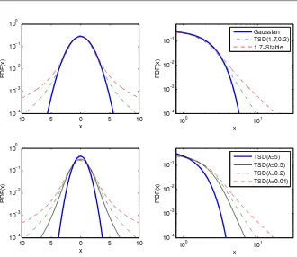
Figure 1.3:Top panels: Semilog and loglog plots of symmetric 1.7-stable, sym-metric tempered stable (TSD) with α = 1.7 and λ = 0.2, and Gaussian pdfs. Bottom panels: Semilog and loglog plots of sym-metric TSD pdfs with α = 1.7 and four truncation coefficients:
λ = 5,0.5,0.2,0.01. Note, that for large λ’s the distribution ap-proaches the Gaussian (though with a different scale) and for small
λ’s the stable law with the same shape parameterα.
STF2stab03.m
The (exponentially smoothed) TLD was not recognized in finance until the introduction of the KoBoL (Boyarchenko and Levendorskii, 2000) and CGMY models (Carr et al., 2002). Around this time Rosinski coined the term under which the exponentially smoothed TLD is known today in the mathematics literature – tempered stable distribution (TSD; see Rosinski, 2007).
Despite the interesting statistical properties, the TSDs (TLDs) have not been applied extensively to date. The most probable reason for this being the com-plicated definition of the TSD. Like for stable distributions, only the charac-teristic function is known. No closed form formulas exist for the density or the distribution functions. No integral formulas, like Zolotarev’s (1986) for the stable laws (see Section 1.2.2), have been discovered to date. Hence, statis-tical inference is, in general, limited to ML utilizing the FFT technique for approximating the pdf (Bianchi et al., 2010; Grabchak, 2008). Moreover, com-pared to the stable distribution, the TSD introduces one more parameter (the truncationλ) making the estimation procedure even more complicated. Other parameter fitting techniques proposed so far comprise a combination ofad hoc
approaches and moment matching (Boyarchenko and Levendorskii, 2000; Mat-acz, 2000). Apart from a few special cases, also the simulation of TSD variables is cumbersome and numerically demanding (Bianchi et al., 2010; Kawai and Masuda, 2010; Poirot and Tankov, 2006).
1.4
Generalized Hyperbolic Distributions
1.4.1
Definitions and Basic Properties
The hyperbolic distribution saw its appearance in finance in the mid-1990s, when a number of authors reported that it provides a very good model for the empirical distributions of daily stock returns from a number of leading German enterprises (Eberlein and Keller, 1995; K¨uchler et al., 1999). Since then it has become a popular tool in stock price modeling and market risk measurement (Bibby and Sørensen, 2003; Chen, H¨ardle and Jeong, 2008; McNeil, R¨udiger and Embrechts, 2005). However, the origins of the hyperbolic law date back to the 1940s and the empirical findings in geophysics. A formal mathematical description was developed years later by Barndorff-Nielsen (1977).
0 0.5 1 1.5 2 0
0.2 0.4 0.6 0.8 1
x
PDF(x)
−10 −5 0 5 10
10−8 10−6 10−4 10−2 100
x
PDF(x)
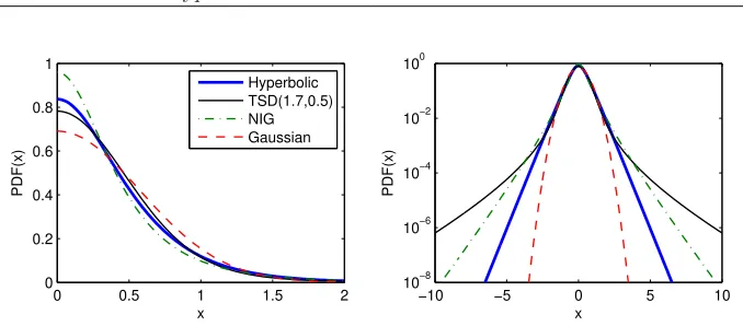
[image:19.595.86.425.123.272.2]Hyperbolic TSD(1.7,0.5) NIG Gaussian
Figure 1.4: Densities and log-densities of symmetric hyperbolic, TSD, NIG, and Gaussian distributions having the same variance, see eqns. (1.18) and (1.33). The name of the hyperbolic distribution is derived from the fact that its log-density forms a hyperbola, which is clearly visible in the right panel.
STF2stab04.m
Section, the hyperbolic law is a member of a larger, versatile class of generalized hyperbolic (GH) distributions, which also includes the normal-inverse Gaussian (NIG) and variance-gamma (VG) distributions as special cases. For a concise review of special and limiting cases of the GH distribution see Chapter 9 in Paolella (2007).
The Hyperbolic Distribution. The hyperbolic distribution is defined as a normal variance-mean mixture where the mixing distribution is the generalized inverse Gaussian (GIG) law with parameterλ= 1, i.e. it is conditionally Gaus-sian (Barndorff-Nielsen, 1977; Barndorff-Nielsen and Blaesild, 1981). More precisely, a random variableZ has the hyperbolic distribution if:
(Z|Y)∼N (µ+βY, Y), (1.20) where Y is a generalized inverse Gaussian GIG(λ = 1, χ, ψ) random variable and N(m, s2) denotes the Gaussian distribution with meanmand variances2.
The GIG law is a positive domain distribution with the pdf given by:
fGIG(x) = (ψ/χ) λ/2
2Kλ(√χψ)x λ−1e−1
2(χx− 1
where the three parameters take values in one of the ranges: (i)χ >0, ψ≥0 if
λ <0, (ii) χ >0, ψ >0 ifλ= 0 or (iii)χ≥0, ψ= 0 ifλ >0. The generalized inverse Gaussian law has a number of interesting properties that we will use later in this section. The distribution of the inverse of a GIG variable is again GIG but with a differentλ, namely if:
Y ∼GIG(λ, χ, ψ) then Y−1∼GIG(−λ, χ, ψ). (1.22) A GIG variable can be also reparameterized by setting a = p
χ/ψ and b =
√
χψ, and definingY =aY˜, where: ˜
Y ∼GIG(λ, b, b). (1.23)
The normalizing constant Kλ(t) in formula (1.21) is the modified Bessel func-tion of the third kind with indexλ, also known as the MacDonald function. It is defined as:
Kλ(t) = 1 2
Z ∞
0
xλ−1e−1 2t(x+x−
1
)dx, t >0. (1.24)
In the context of hyperbolic distributions, the Bessel functions are thoroughly discussed in Barndorff-Nielsen and Blaesild (1981). Here we recall only two properties that will be used later. Namely, (i) Kλ(t) is symmetric with respect to λ, i.e. Kλ(t) = K−λ(t), and (ii) forλ=±12 it can be written in a simpler
form:
K±1 2(t) =
r
π
2t
−1
2e−t. (1.25)
Relation (1.20) implies that a hyperbolic random variable Z ∼ H(ψ, β, χ, µ) can be represented in the form: Z∼µ+βY +√YN(0,1), with the cf:
φZ(u) =eiuµ
Z ∞
0
eiβzu−12zu 2
dFY(z). (1.26)
HereFY(z) denotes the distribution function of a GIG random variableY with parameterλ= 1, see eqn. (1.21). Hence, the hyperbolic pdf is given by:
fH(x;ψ, β, χ, µ) =
p
ψ/χ
2p
ψ+β2K
1(√ψχ)
e−√{ψ+β2}{χ+(x−µ)2}+β(x−µ), (1.27)
or in an alternative parameterization (withδ=√χ andα=p
ψ+β2) by:
fH(x;α, β, δ, µ) =
p
α2−β2
2αδK1(δ p
α2−β2)e
−α√δ2+(x−µ)2+β(x−µ)
The latter is more popular and has the advantage ofδ >0 being the traditional scale parameter. Out of the remaining three parameters,α and β determine the shape, with α being responsible for the steepness and 0 ≤ |β| < α for the skewness, and µ ∈ R is the location parameter. Finally, note that if we only have an efficient algorithm to compute K1, the calculation of the pdf is
straightforward. However, the cdf has to be numerically integrated from (1.27) or (1.28).
The General Class. The generalized hyperbolic (GH) law can be represented as a normal variance-mean mixture where the mixing distribution is the gen-eralized inverse Gaussian law with anyλ∈R. Hence, the GH distribution is described by five parametersθ= (λ, α, β, δ, µ), using parameterization (1.28), and its pdf is given by:
fGH(x;θ) =κ
δ2+ (x−µ)2
1 2(λ−
1 2)
Kλ−1 2
αpδ2+ (x−µ)2eβ(x−µ),
(1.29) where:
κ= (α
2−β2)λ
2 √
2παλ−1 2δλKλ(δ
p
α2−β2). (1.30)
The tail behavior of the GH density is ‘semi-heavy’, i.e. the tails are lighter than those of non-Gaussian stable laws and TSDs with a relatively small truncation parameter (see Figure 1.4), but much heavier than Gaussian. Formally, the following asymptotic relation is satisfied (Barndorff-Nielsen and Blaesild, 1981):
fGH(x)≈ |x|λ−1e(∓α+β)x for x→ ±∞, (1.31) which can be interpreted as exponential ‘tempering’ of the power-law tails (compare with the TSD described in Section 1.3). Consequently, all moments of the GH law exist. In particular, the mean and variance are given by:
E(X) = µ+βδ
2
ζ
Kλ+1(ζ)
Kλ(ζ) , (1.32)
Var(X) = δ2
"
Kλ+1(ζ)
ζKλ(ζ) +
β2δ2
ζ2 (
Kλ+2(ζ)
Kλ(ζ) −
Kλ
+1(ζ)
ζKλ(ζ)
2)#
.(1.33)
The Normal-Inverse Gaussian Distribution. The normal-inverse
Gaus-sian (NIG) laws were introduced by Barndorff-Nielsen (1995) as a subclass of the generalized hyperbolic laws obtained forλ=−1
distribution is given by:
fNIG(x) = αδ
π e
δ√α2−β2+β(x−µ)K1(α
p
δ2+ (x−µ)2) p
δ2+ (x−µ)2 . (1.34)
Like for the hyperbolic law the calculation of the pdf is straightforward, but the cdf has to be numerically integrated from eqn. (1.34).
At the expense of four parameters, the NIG distribution is able to model asym-metric distributions with ‘semi-heavy’ tails. However, if we letα→0 the NIG distribution converges to the Cauchy distribution (with location parameter
µ and scale parameter δ), which exhibits extremely heavy tails. Obviously, the NIG distribution may not be adequate to deal with cases of extremely heavy tails such as those of Pareto or non-Gaussian stable laws. However, empirical experience suggests excellent fits of the NIG law to financial data (Karlis, 2002; Karlis and Lillest¨ol, 2004; Venter and de Jongh, 2002).
Moreover, the class of normal-inverse Gaussian distributions possesses an ap-pealing feature that the class of hyperbolic laws does not have. Namely, it is closed under convolution, i.e. a sum of two independent NIG random vari-ables is again NIG (Barndorff-Nielsen, 1995). In particular, if X1 and X2
are independent NIG random variables with common parametersαandβ but having different scale and location parametersδ1,2 andµ1,2, respectively, then
X =X1+X2 is NIG(α, β, δ1+δ1, µ1+µ2). Only two subclasses of the GH
distributions are closed under convolution. The other class with this important property is the class of variance-gamma (VG) distributions, which is obtained when δ is equal to 0. This is only possible for λ > 0 and α > |β|. The VG distributions (with β = 0) were introduced to finance by Madan and Seneta (1990), long before the popularity of GH and NIG laws.
1.4.2
Simulation of Generalized Hyperbolic Variables
The most natural way of simulating GH variables is derived from the property that they can be represented as normal variance-mean mixtures. Since the mixing distribution is the GIG law, the resulting algorithm reads as follows:
1. simulate a random variableY ∼GIG(λ, χ, ψ) = GIG(λ, δ2, α2−β2);
The algorithm is fast and efficient if we have a handy way of simulating GIG variates. Forλ=−12, i.e. when sampling from the so-called inverse Gaussian
(IG) distribution, there exists an efficient procedure that utilizes a transforma-tion yielding two roots. It starts with the observatransforma-tion that if we letϑ=p
χ/ψ
then the IG(χ, ψ) density (= GIG(−12, χ, ψ); see eqn. (1.21)) of Y can be
written as:
fIG(x) =
r
χ
2πx3exp
−χ(x−ϑ)2
2xϑ2
. (1.35)
Now, following Shuster (1968) we may write:
V = χ(Y −ϑ)
2
Y ϑ2 ∼χ 2
(1), (1.36)
i.e. V is distributed as a chi-square random variable with one degree of freedom. As such it can be simply generated by taking a square of a standard normal random number. Unfortunately, the value ofY is not uniquely determined by eqn. (1.36). Solving this equation forY yields two roots:
y1=ϑ+ ϑ
2χ
ϑV −p4ϑχV +ϑ2V2 and y
2=ϑ
2
y1.
The difficulty in generating observations with the desired distribution now lies in choosing between the two roots. Michael, Schucany and Haas (1976) showed that Y can be simulated by choosing y1 with probability ϑ/(ϑ+y1). So for
each random observationV from aχ2
(1) distribution the smaller rooty1has to
be calculated. Then an auxiliary Bernoulli trial is performed with probability
p=ϑ/(ϑ+y1). If the trial results in a ‘success’, y1 is chosen; otherwise, the
larger rooty2is selected. This routine is, for instance, implemented in thernig
function of the Rmetrics collection of software packages for S-plus/R (see also Section 1.2.2 where Rmetrics was briefly described).
In the general case, the GIG distribution – as well as the (generalized) hyper-bolic law – can be simulated via the rejection algorithm. An adaptive version of this technique is used to obtain hyperbolic random numbers in the rhyp
This difficulty led to a search for a short algorithm which would give comparable efficiencies but without the drawback of extensive numerical optimizations. A solution, based on the ‘ratio-of-uniforms’ method, was provided by Dagpunar (1989). First, recalling properties (1.22) and (1.23), observe that we only need to find a method to simulate ˜Y ∼ GIG(λ, b, b) variables and only for non-negativeλ’s. Next, define the relocated variable ˜Ym= ˜Y −m, where the shift
m= 1b(λ−1 +p(λ−1)2+b2) is the mode of the density of ˜Y. Then ˜Y can be
generated by setting ˜Ym=V /U, where the pair (U, V) is uniformly distributed over the region{(u, v) : 0≤u≤p
h(v/u)} with:
h(t) = (t+m)λ−1exp
−b
2
t+m+ 1
t+m
, for t≥ −m.
Since this region is irregularly shaped, it is more convenient to generate the pair (U, V) uniformly over a minimal enclosing rectangle{(u, v) : 0≤u≤u+,
v− ≤v ≤v+}. Finally, the variate (V /U) is accepted ifU2 ≤h(V /U). The
efficiency of the algorithm depends on the method of deriving and the actual choice ofu+andv±. Further, forλ≤1 andb≤1 there is no need for the shift
at mode m. Such a version of the algorithm is implemented in UNU.RAN, a library of C functions for non-uniform random number generation developed at the Vienna University of Economics, see statistik.wu-wien.ac.at/unuran.
1.4.3
Estimation of Parameters
Maximum Likelihood Method. The parameter estimation of GH
distri-butions can be performed by the ML method, since there exist closed-form formulas (although, involving special functions) for the densities of these laws. The computational burden is not as heavy as for stable laws, but it still is considerable. In general, the ML estimation algorithm is as follows. For a vec-tor of observations x= (x1, ..., xn), the ML estimate of the parameter vector
θ= (λ, α, β, δ, µ) is obtained by maximizing the log-likelihood function:
L(x;θ) = logκ+λ−
1 2
2 n
X
i=1
log(δ2+ (xi−µ)2) +
+ n
X
i=1
log Kλ−1 2(α
p
δ2+ (x
i−µ)2) + n
X
i=1
β(xi−µ), (1.37)
The routines proposed in the literature differ in the choice of the optimiza-tion scheme. The first software product that allowed statistical inference with hyperbolic distributions, the HYP program, used a gradient search technique (Blaesild and Sorensen, 1992). In a large simulation study Prause (1999) uti-lized the bracketing method. Matlab functions hypest.m and nigest.m dis-tributed with the MFE Toolbox (Weron, 2006) use the downhill simplex method, with slight modifications due to parameter restrictions.
The main factor for the speed of the estimation is the number of modified Bessel functions to compute. Note, that forλ= 1 (i.e. the hyperbolic distribution) this function appears only in the constantκ. For a data set withnindependent observations we need to evaluatenandn+ 1 Bessel functions for NIG and GH distributions, respectively, whereas only one for the hyperbolic. This leads to a considerable reduction in the time necessary to calculate the likelihood function in the hyperbolic case. Prause (1999) reported a reduction of ca. 33%, however, the efficiency results are highly sample and implementation dependent.
We also have to say that the optimization is challenging. Some of the param-eters are hard to separate since a flat-tailed GH distribution with a large scale parameter is hard to distinguish from a fat-tailed distribution with a small scale parameter, see Barndorff-Nielsen and Blaesild (1981) who observed such a behavior already for the hyperbolic law. The likelihood function with respect to these parameters then becomes very flat, and may have local minima. In the case of NIG distributions Venter and de Jongh (2002) proposed simple esti-mates ofαandβthat can be used as staring values for the ML scheme. Starting from relation (1.31) for the tails of the NIG density (i.e. withλ=−1/2) they derived the following approximation:
α−β ∼ 12 x1−f+E(X|X > x1−f)
E(X2|X > x
1−f)−x1−fE(X|X > x1−f)
,
α+β ∼ −12 xf +E(X|X < xf)
E(X2|X < x
f)−xfE(X|X < xf)
,
wherexf is thef-th population quantile, see Section 1.2.4. After the choice of a suitable value forf, Venter and de Jongh usedf = 5%, the ‘tail estimates’ ofαand β are obtained by replacing the quantiles and expectations by their sample values in the above relations.
Another method of providing the starting values for the ML scheme was sug-gested by Prause (1999). He estimated the parameters of a symmetric (β =
Other Methods. Besides the ML approach other estimation methods have been proposed in the literature. Prause (1999) tested different estimation tech-niques by replacing the log-likelihood function with other score functions, like the Anderson-Darling and Kolmogorov statistics or Lp-norms. But the re-sults were disappointing. Karlis and Lillest¨ol (2004) made use of the MCMC technique, however, again the results obtained were not impressive. Karlis (2002) described an Expectation-Maximization (EM) type algorithm for ML estimation of the NIG distribution. The algorithm can be programmed in any statistical package supporting Bessel functions and it has all the properties of the standard EM algorithm, like sure, but slow, convergence, parameters in the admissible range, etc. Recently Fragiadakis, Karlis and Meintanis (2009) used this approach to construct goodness-of-fit tests for symmetric NIG distribu-tions. The tests are based on a weighted integral incorporating the empirical cf of suitably standardized data. The EM scheme can be also generalized to multivariate GH distributions (but with fixedλ, see Protassov, 2004).
1.5
Empirical Evidence
The empirical facts presented in Section 1.1 show that we should use heavy tailed alternatives to the Gaussian law in order to obtain acceptable estimates of market losses. In this section we apply the techniques discussed so far to two samples of financial data: the Dow Jones Industrial Average (DJIA) index and the Polish WIG20 index. Both are blue chip stock market indexes. DJIA is composed of 30 major U.S. companies that trade on NYSE and NASDAQ. WIG20 consists of 20 major Polish companies listed on the Warsaw Stock Exchange. We use daily closing index values from the period January 3, 2000 – December 31, 2009. Eliminating missing values (mostly U.S. and Polish holidays) we end up with 2494 (log-)returns for each index, see the top left panels in Figures 1.5 and 1.6.
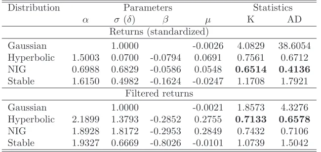
Table 1.1: Gaussian, hyperbolic, NIG, and stable fits to 2516 standardized (rescaled by the sample standard deviation) andσt-filtered returns of the DJIA from the period January 3, 2000 – December 31, 2009, see also Figure 1.5. The values of the Kolmogorov (K) and Anderson-Darling (AD) goodness-of-fit statistics suggest the hyperbolic and NIG distributions as the best models for filtered and standardized returns, respectively.
Distribution Parameters Statistics
α σ(δ) β µ K AD Returns (standardized)
Gaussian 1.0000 -0.0026 4.0829 38.6054
Hyperbolic 1.5003 0.0700 -0.0794 0.0691 0.7561 0.6712
NIG 0.6988 0.6829 -0.0586 0.0548 0.6514 0.4136
Stable 1.6150 0.4982 -0.1624 -0.0247 1.1708 1.7921
Filtered returns
Gaussian 1.0000 -0.0021 1.8573 4.3276
Hyperbolic 2.1899 1.3793 -0.2852 0.2755 0.7133 0.6578
NIG 1.8928 1.8172 -0.2953 0.2849 0.7432 0.7106
Stable 1.9327 0.6669 -0.8026 -0.0101 1.0739 1.5042
a GARCH(1,1) process:
rt=σtǫt, with σt=c0+c1rt2−1+d1σt2−1, (1.38)
wherec0,c1andd1 are constants and
ǫt= rt
σt
, (1.39)
are the filtered returns, see the top right panels in Figures 1.5 and 1.6. We could also insert a moving average term in the conditional mean to remove any serial dependency if needed.
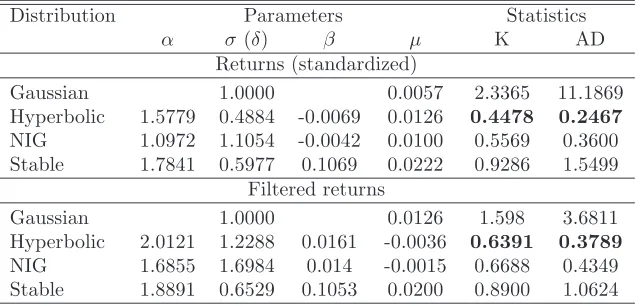
Table 1.2: Gaussian, hyperbolic, NIG and stable fits to 2514 standardized (rescaled by the sample standard deviation) and σt-filtered returns of the Polish WIG20 index from the period January 3, 2000 – Decem-ber 31, 2009, see also Figure 1.6. The values of the Kolmogorov (K) and Anderson-Darling (AD) goodness-of-fit statistics suggest the hy-perbolic distribution as the best model, with the NIG law following closely by.
Distribution Parameters Statistics
α σ(δ) β µ K AD Returns (standardized)
Gaussian 1.0000 0.0057 2.3365 11.1869
Hyperbolic 1.5779 0.4884 -0.0069 0.0126 0.4478 0.2467
NIG 1.0972 1.1054 -0.0042 0.0100 0.5569 0.3600
Stable 1.7841 0.5977 0.1069 0.0222 0.9286 1.5499
Filtered returns
Gaussian 1.0000 0.0126 1.598 3.6811
Hyperbolic 2.0121 1.2288 0.0161 -0.0036 0.6391 0.3789
NIG 1.6855 1.6984 0.014 -0.0015 0.6688 0.4349
Stable 1.8891 0.6529 0.1053 0.0200 0.8900 1.0624
0 500 1000 1500 2000 2500 −0.1 −0.05 0 0.05 0.1 Days (2000.01.03−2009.12.31) Returns
0 500 1000 1500 2000 2500 −6 −4 −2 0 2 4 6 Days (2000.01.03−2009.12.31) Returns Returns σ
Filtered DJIA returns
100 101 10−4 10−3 10−2 10−1 −x CDF(x)
100 101 10−4 10−3 10−2 10−1 x 1−CDF(x)
100 101 10−4 10−3 10−2 10−1 −x CDF(x)
[image:29.595.90.421.132.532.2]100 101 10−4 10−3 10−2 10−1 x 1−CDF(x) Returns Gauss Hyp NIG Stable Returns Gauss Hyp NIG Stable Filt. returns Gauss Hyp NIG Stable Filt. returns Gauss Hyp NIG Stable
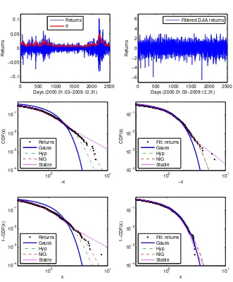
Figure 1.5:Top left: DJIA index (log-)returns and the GARCH(1,1)-based daily volatility estimate σt. Top right: σt-filtered DJIA returns.
Middle: The left tails of the cdf of (standardized) returns (left) or filtered returns (right) and of four fitted distributions. Bottom: The corresponding right tails.
0 500 1000 1500 2000 2500 −0.1 −0.05 0 0.05 0.1 Days (2000.01.03−2009.12.31) Returns Returns σ
0 500 1000 1500 2000 2500 −6 −4 −2 0 2 4 6 Days (2000.01.03−2009.12.31) Returns
Filtered WIG20 returns
100 101 10−4 10−3 10−2 10−1 −x CDF(x) Returns Gauss Hyp NIG Stable
100 101 10−4 10−3 10−2 10−1 x 1−CDF(x) Returns Gauss Hyp NIG Stable
100 101 10−4
10−3 10−2 10−1
−x CDF(x) Filt. returns
Gauss Hyp NIG Stable
100 101 10−4
10−3 10−2 10−1
x 1−CDF(x) Filt. returns
[image:30.595.173.507.117.534.2]Gauss Hyp NIG Stable
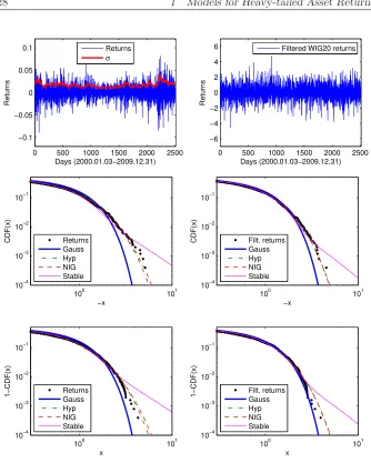
Figure 1.6:Top left: WIG20 index (log-)returns and the GARCH(1,1)-based daily volatility estimate σt. Top right: σt-filtered WIG20 returns.
Middle: The left tails of the cdf of (standardized) returns (left) or filtered returns (right) and of four fitted distributions. Bottom: The corresponding right tails.
Atkinson, A. C. (1982). The simulation of generalized inverse Gaussian and hy-perbolic random variables,SIAM Journal of Scientific & Statistical Com-puting3: 502–515.
Barndorff-Nielsen, O. E. (1977). Exponentially decreasing distributions for the logarithm of particle size,Proceedings of the Royal Society London A353: 401–419.
Barndorff-Nielsen, O. E. (1995). Normal\\Inverse Gaussian Processes and the Modelling of Stock Returns, Research Report 300, Department of Theo-retical Statistics, University of Aarhus.
Barndorff-Nielsen, O. E. and Blaesild, P. (1981). Hyperbolic distributions and ramifications: Contributions to theory and applications,in C. Taillie, G. Patil, B. Baldessari (eds.)Statistical Distributions in Scientific Work, Vol-ume 4, Reidel, Dordrecht, pp. 19–44.
Barone-Adesi, G., Giannopoulos, K., and Vosper, L., (1999). VaR without cor-relations for portfolios of derivative securities,Journal of Futures Markets 19(5): 583–602.
Basle Committee on Banking Supervision (1995). An internal model-based approach to market risk capital requirements, http://www.bis.org.
Bianchi, M. L., Rachev, S. T., Kim, Y. S. and Fabozzi, F. J. (2010). Tempered stable distributions and processes in finance: Numerical analysis, in M. Corazza, P. Claudio, P. (Eds.)Mathematical and Statistical Methods for Actuarial Sciences and Finance, Springer.
Bibby, B. M. and Sørensen, M. (2003). Hyperbolic processes in finance, in
Blaesild, P. and Sorensen, M. (1992).HYP – a Computer Program for Analyz-ing Data by Means of the Hyperbolic Distribution, Research Report 248, Department of Theoretical Statistics, Aarhus University.
Boyarchenko, S. I. and Levendorskii, S. Z. (2000). Option pricing for truncated L´evy processes,International Journal of Theoretical and Applied Finance 3: 549–552.
Brcich, R. F., Iskander, D. R. and Zoubir, A. M. (2005). The stability test for symmetric alpha stable distributions, IEEE Transactions on Signal Processing53: 977–986.
Buckle, D. J. (1995). Bayesian inference for stable distributions,Journal of the American Statistical Association90: 605–613.
Carr, P., Geman, H., Madan, D. B. and Yor, M. (2002). The fine structure of asset returns: an empirical investigation,Journal of Business75: 305–332.
Chambers, J. M., Mallows, C. L. and Stuck, B. W. (1976). A Method for Simulating Stable Random Variables,Journal of the American Statistical Association71: 340–344.
Chen, Y., H¨ardle, W. and Jeong, S.-O. (2008). Nonparametric risk manage-ment with generalized hyperbolic distributions, Journal of the American Statistical Association103: 910–923.
Cont, R., Potters, M. and Bouchaud, J.-P. (1997). Scaling in stock market data: Stable laws and beyond, in B. Dubrulle, F. Graner, D. Sornette (eds.)Scale Invariance and Beyond, Proceedings of the CNRS Workshop on Scale Invariance, Springer, Berlin.
D’Agostino, R. B. and Stephens, M. A. (1986). Goodness-of-Fit Techniques, Marcel Dekker, New York.
Dagpunar, J. S. (1989). An Easily Implemented Generalized Inverse Gaussian Generator,Communications in Statistics – Simulations18: 703–710.
Danielsson, J., Hartmann, P. and De Vries, C. G. (1998). The cost of conser-vatism: Extreme returns, value at risk and the Basle multiplication factor,
Risk11: 101–103.
Dominicy, Y. and Veredas, D. (2010). The method of simulated quantiles,
DuMouchel, W. H. (1971). Stable Distributions in Statistical Inference, Ph.D. Thesis, Department of Statistics, Yale University.
DuMouchel, W. H. (1973). On the Asymptotic Normality of the Maximum– Likelihood Estimate when Sampling from a Stable Distribution, Annals of Statistics1(5): 948–957.
Eberlein, E. and Keller, U. (1995). Hyperbolic distributions in finance,
Bernoulli1: 281–299.
Fama, E. F. and Roll, R. (1971). Parameter Estimates for Symmetric Stable Distributions, Journal of the American Statistical Association 66: 331– 338.
Fan, Z. (2006). Parameter estimation of stable distributions,Communications in Statistics – Theory and Methods35(2): 245–255.
Fragiadakis, K., Karlis, D. and Meintanis, S. G. (2009). Tests of fit for normal inverse Gaussian distributions,Statistical Methodology6: 553–564.
Garcia, R., Renault, E. and Veredas, D. (2010). Estimation of stable distribu-tions by indirect inference,Journal of Econometrics, Forthcoming.
Grabchak, M. (2010). Maximum likelihood estimation of parametric tempered stable distributions on the real line with applications to finance, Ph.D. thesis, Cornell University.
Grabchak, M. and Samorodnitsky, G. (2010). Do financial returns have finite or infinite variance? A paradox and an explanation,Quantitative Finance, DOI: 10.1080/14697680903540381.
Guillaume, D. M., Dacorogna, M. M., Dave, R. R., M¨uller, U. A., Olsen, R. B. and Pictet, O. V. (1997). From the birds eye to the microscope: A survey of new stylized facts of the intra-daily foreign exchange markets,Finance & Stochastics1: 95–129.
Janicki, A. and Weron, A. (1994a). Can one see α-stable variables and pro-cesses,Statistical Science9: 109–126.
Janicki, A. and Weron, A. (1994b). Simulation and Chaotic Behavior of α -Stable Stochastic Processes, Marcel Dekker.
Karlis, D. and Lillest¨ol, J. (2004). Bayesian estimation of NIG models via Markov chain Monte Carlo methods, Applied Stochastic Models in Busi-ness and Industry20(4): 323–338.
Kawai, R. and Masuda, H. (2010). On simulation of tempered stable random variates,Preprint, Kyushu University.
Kogon, S. M. and Williams, D. B. (1998). Characteristic function based esti-mation of stable parameters,in R. Adler, R. Feldman, M. Taqqu (eds.),
A Practical Guide to Heavy Tails, Birkhauser, pp. 311–335.
Koponen, I. (1995). Analytic approach to the problem of convergence of trun-cated Levy flights towards the Gaussian stochastic process, Physical Re-view E52: 1197–1199.
Koutrouvelis, I. A. (1980). Regression–Type Estimation of the Parameters of Stable Laws,Journal of the American Statistical Association75: 918–928.
Kuester, K., Mittnik, S., and Paolella, M.S. (2006). Value-at-Risk prediction: A comparison of alternative strategies,Journal of Financial Econometrics 4(1): 53–89.
K¨uchler, U., Neumann, K., Sørensen, M. and Streller, A. (1999). Stock returns and hyperbolic distributions,Mathematical and Computer Modelling 29: 1–15.
Lombardi, M. J. (2007). Bayesian inference forα-stable distributions: A ran-dom walk MCMC approach,Computational Statistics and Data Analysis 51(5): 2688–2700.
Madan, D. B. and Seneta, E. (1990). The variance gamma (V.G.) model for share market returns,Journal of Business 63: 511–524.
Mandelbrot, B. B. (1963). The variation of certain speculative prices,Journal of Business36: 394–419.
Mantegna, R. N. and Stanley, H. E. (1994). Stochastic processes with ultraslow convergence to a Gaussian: The truncated L´evy flight, Physical Review Letters73: 2946–2949.
Matsui, M. and Takemura, A. (2006). Some improvements in numerical evalu-ation of symmetric stable density and its derivatives,Communications in Statistics – Theory and Methods35(1): 149–172.
Matsui, M. and Takemura, A. (2008). Goodness-of-fit tests for symmetric stable distributions – empirical characteristic function approach, TEST 17(3): 546–566.
McCulloch, J. H. (1986). Simple consistent estimators of stable distribution parameters,Communications in Statistics – Simulations15: 1109–1136.
McNeil, A. J., R¨udiger, F. and Embrechts, P. (2005). Quantitative Risk Man-agement, Princeton University Press, Princeton, NJ.
Michael, J. R., Schucany, W. R. and Haas, R. W. (1976). Generating Ran-dom Variates Using Transformations with Multiple Roots,The American Statistician30: 88–90.
Mittnik, S., Doganoglu, T. and Chenyao, D. (1999). Computing the Probability Density Function of the Stable Paretian Distribution, Mathematical and Computer Modelling 29: 235–240.
Mittnik, S. and Paolella, M. S. (1999). A simple estimator for the characteristic exponent of the stable Paretian distribution,Mathematical and Computer Modelling29: 161–176.
Mittnik, S., Rachev, S. T., Doganoglu, T. and Chenyao, D. (1999). Maxi-mum Likelihood Estimation of Stable Paretian Models,Mathematical and Computer Modelling 29: 275–293.
Nolan, J. P. (1997). Numerical Calculation of Stable Densities and Distribution Functions,Communications in Statistics – Stochastic Models13: 759–774.
Nolan, J. P. (2001). Maximum Likelihood Estimation and Diagnostics for Stable Distributions, in O. E. Barndorff-Nielsen, T. Mikosch, S. Resnick (eds.),L´evy Processes, Brikh¨auser, Boston.
Nolan, J. P. (2010). Stable Distributions – Models for Heavy
Tailed Data, Birkh¨auser, Boston. In progress, Chapter 1 online at academic2.american.edu/∼jpnolan.
Paolella, M. S. (2001). Testing the stable Paretian assumption, Mathematical and Computer Modelling34: 1095–1112.
Paolella, M. S. (2007). Intermediate Probability: A Computational Approach, Wiley, Chichester.
Peters, G. W., Sisson, S. A. and Fan, Y. (2009). Likelihood-free Bayesian inference forα-stable models,Preprint: http://arxiv.org/abs/0912.4729. Poirot, J. and Tankov, P. (2006). Monte Carlo option pricing for tempered
stable (CGMY) processes, Asia-Pacific Financial Markets 13(4): 327-344.
Prause, K. (1999). The Generalized Hyperbolic Model: Estimation, Finan-cial Derivatives, and Risk Measures, Ph.D. Thesis, Freiburg University, http://www.freidok.uni-freiburg.de/volltexte/15.
Press, S. J. (1972). Estimation in Univariate and Multivariate Stable Distri-bution,Journal of the American Statistical Association 67: 842–846.
Protassov, R. S. (2004). EM-based maximum likelihood parameter estimation for multivariate generalized hyperbolic distributions with fixedλ, Statis-tics and Computing14: 67–77.
Rachev, S. and Mittnik, S. (2000). Stable Paretian Models in Finance, Wiley.
Rosinski, J. (2007). Tempering stable processes,Stochastic Processes and Their Applications117(6): 677–707.
Ross, S. (2002). Simulation, Academic Press, San Diego.
Samorodnitsky, G. and Taqqu, M. S. (1994). Stable Non–Gaussian Random Processes, Chapman & Hall.
Shuster, J. (1968). On the Inverse Gaussian Distribution Function,Journal of the American Statistical Association63: 1514–1516.
Stahl, G. (1997). Three cheers,Risk10: 67–69.
Stute, W., Manteiga, W. G. and Quindimil, M.P. (1993). Bootstrap Based Goodness-Of-Fit-Tests,Metrika40: 243–256.
Weron, R. (1996). On the Chambers-Mallows-Stuck Method for Simulat-ing Skewed Stable Random Variables, Statistics and Probability Let-ters 28: 165–171. See also R. Weron (1996) Correction to: On the Chambers-Mallows-Stuck Method for Simulating Skewed Stable Random Variables, Working Paper, Available at MPRA: http://mpra.ub.uni-muenchen.de/20761/.
Weron, R. (2001). Levy–Stable Distributions Revisited: Tail Index>2 Does Not Exclude the Levy–Stable Regime, International Journal of Modern Physics C12: 209–223.
Weron, R. (2004). Computationally Intensive Value at Risk Calculations, in
J. E. Gentle, W. H¨ardle, Y. Mori (eds.)Handbook of Computational Statis-tics, Springer, Berlin, 911–950.
Weron, R. (2006). Modeling and Forecasting Electricity Loads and Prices: A Statistical Approach, Wiley, Chichester.
Zolotarev, V. M. (1964). On representation of stable laws by integrals,Selected Translations in Mathematical Statistics and Probability 4: 84–88.