Jet Pumps EUR 3253

'$Hï

-«■ivri£ ÏHSMIIW itiisi!

m

mmm

EUROPEAN ATOMIC ENERGY COMMUNITY - EURATOM REACTOR CENTRUM NEDERLAND - RCN

•$m.

m

i f l J E T P U M P

.ιΐΛί im

M

J.T. WILM

la*: ••»»MW

«·?.·

ÍM

1

*

Æ?

Ä«

M K

I l t · « * * ! ;

w*ï »Λί

W 1966

'»ΜΗ

flu?.

•-..»ι

i

Ä

M M · «

p i

îlfeîv

i^rv*

¡i«w

i'rTV·

►''■»'P

l!«H

SÉM

»H* «tn!

MUI

*I

i»·

«»•il _JtPr'

Ig

Äff

wáwJsPp^

s

«UM tttiii

s i l PW' 'ir"^"!···*4 p"^»Pr

¿Ai

1

RU'

ÍM

U:\

W W'jfli

II

Aili

m Ai

This document was prepared under the sponsorship of the Commission of the European Atomic Enerfry Community (EURATOM).

any person

îïmâ

'■».¿rotó ifli&ifflHM |C"S "

accuracy, completeness, or usefulness of the information con-in this document, or t h a t the use of any con-information, apparatus,

I o r riroc.ess disclosed in t h i s d o c u m e n t m a v n o t infringe

Neither the EURATOM Commission, its contractors nor acting on their behalf

Make any warranty or representation, express or implied, with respe to the

tained in

method, or process disclosed in this document may not infringe privately owned rights; or

Assume any liability with respect to the use of, or for damages resulting

iiii

ΛΙ

a t the price of F F 8.50 F B 85,— DM 6.80 Lit. 1.060 Fl. 6.20

ttriÜ

«

When ordening, please quote the EUR n u m b e r and the title, which are indicated on the cover of each report.

lift!

E U R 3 2 5 3 . e

EUROPEAN ATOMIC ENERGY COMMUNITY - EURATOM REACTOR CENTRUM NEDERLAND - RCN

J E T P U M P S

by

J.T. WILMAN (RCN)

1966

The present publication is one of a series giving more detailed information on special subjects covered under the NERO development programme carried out by the Reac-tor Centrum Nederland in association with Euratom

(Contract No. 007-61-6 PNIN).

A general description of the design data and the experimental work, which is aimed at the development of a pressurized-water reactor for marine application, is given in Euratom Reports:

"EUR 2180.e - NERO DEVELOPMENT PROGRAMME

Report covering the period January I963 through June 1964"

"EUR 3125.e - NERO DEVELOPMENT PROGRAMME

Report covering the period of July 1964 to December I965"

F O R E W O R D

Jet pumps are basically simple in construction and have no moving parts: in many cases they can be effectively used where the service conditions make it impractical to use mechanical pumps.

As it may also be advantageous to use jet pumps in nuclear reactor cooling systems with internal re-circulation a study of jet pump behaviour was carried out under a research contract with the European Atonic Energy Community (Contract no 007-61-6 PNIN; NERO

development programme, Reactor Centrum Nederland -Euratom).

The results of this study are presented in this report.

SUMMARY

JET PUMPS

CONTENTS

Page

A. INTRODUCTION 6

Β. THE JET PUMP 6

C. DERIVATION OF THE EQUATION REPRESENTING THE RELATIONSHIP BETV/EEN THE TOTAL PRESSURE

RATIO AND THE MASS FLOW RATIO (Figure 1) 7

D, THE THEORETICAL JET PUMP CHARACTERISTIC 14

S. THE EFFICIENCY OF A JET PUMP (Figure 2) 15

F. THE EXPERIMENTAL EQUIPMENT (Figures 3 and 4) 17

G. THE TEST (Figure 5) 20

H. TEST RESULTS (Table 1, figures 6 to 16) 22

I. EVALUATION OF THE THEORETICAL

LOSS COEFFICIENTS 26 1.1. Evaluation of Κ ' 2 6

1.2. Evaluation of K, 3 0

1.3. Evaluation of Κ and K. 32

J. CHARACTERISTICS AND

MAXIMUM EFFICIENCY (Figures 17 to 20) 33

K. DETERMINATION OF ABSOLUTE DIMENSIONS 37

L. CONCLUSIONS 4 1

ACKNOWLEDGEMENT 42

CONTENTS (continued)

APPENDIX

1. Reduction of the test data 1.1. Pressure losses

1.2. Mass flow rates 1.3. The mass flow ratio 1.4. Velocities

1.5. The total pressure ratio 1.6. Significant data

2. Tables 2 to 13

Page

43

43 43 46 48 49

J E T P U M P S

A. INTRODUCTION (*)

An attempt was made to derive an equation by means of which the behaviour of jet pumps can be predicted.

To verify the theoretical results a low pressure, low temperature, experimental unit, having a jet pump as principal component, was designed and constructed. A test was performed at the Laboratory of Hydrodynamics at

Delft Technological University.

With the object of optimizing jet pump performance tiie effects of internal changes to the experimental jet pump were also determined.

B. THE JET PUMP

A jet pump (figure 1) is a device in which a fluid flows through a driving nozzle which converts the fluid pressure into a high-velocity jet stream; fluid is continuously entrained from the suction section of the jet pump by the jet stream emerging from the nozzle. In the mixing tube the entrained fluid acquires part of the energy of the motive fluid. In the diffuser the velocity of the mixture is reconverted to pressure.

7

-C. DE.M VATIO?) Ol'1 THE EQUATiOfi JSruEUENTIUG TAIL RELAT I ON,'UTI Ρ

BET7/EEN THE TOTAL PREoSURE RATIO AITO THE MASS FLOW RATIO

A generalized representation of a jet pump is shown in figure 1.

In this figure the planes A, B, 'V, Ζ and C are perpendicular to the axis of the jet pump;

A is a plane just iipstream from the driving nozzle, B is a plane in the suction section of the jet pump, 'r7 is a plane just downstream from the nozzle

discharge tip,

Ζ is a plane at the inlet end of the diffuser, C is a plane at the outlet end of the diffuser.

If it is assumed that in a steady state the static pressure has the same value at all points in the plane W, then (Bernoulli's equation)

P A - P77

=

-?s(n

A

- %) - i ç ( v | - v

2

) +

κ

3

.ίψΙ

,

?B

- %

= - \ ^ΩΒ

- * v - ^ n v

B

- v

2

'

where

PB - % = - ^ s ( hB - h^) - - ^ ( v | - v2) + Kt.;;^v^

p. is the static pressure in the plane A, p-a is the static pressure in the plane B, pv, is the static pressure in the plane W, o is the density of the fluid,

g is the acceleration due to gravity,

h, is the height of A above a reference level 0-0, h-, is the height of Β above the reference level 0-0, h,., is the height of W above the reference level 0-0,

ν is the fluid velocity in the nozzle discharge tip,

s

v. is the velocity of the entrained fluid in the plane W (suction annulus),

Κ is a loss coefficient which applies to the flow

s

between the planes A and W,

K. is a loss coefficient which applies to the flow between the planes Β and W.

The assumption is made that in the plane W just downstream from the nozzle tip the total effective flow area is equal to the cross-sectional area of the mixing tube.

As the jet stream and the suction stream mix

between the plane W and the plane Ζ at the outlet end of the mixing tube (figure 1), it follows from a consideration

of the. change in momentum between the planes W and Ζ that in a steady state, to a good approximation,

(G1 + G2)vz - Gl V g - G2vt =

= CPw - Pz>

S

m

+

f

(h

W -

h

Z

)S

mS " V * p

V

Z

S

m >

where

G1 is the mass flow rate in the driving nozzle, Gp is the mass flow rate in the suction section of

the jet pump,

pz is the static pressure in the plane Z,

hr, is the height of Ζ above the reference level 0-0, vz is the fluid velocity in the plane Z,

S is the cross-sectional area of the mixing tube, Κ is a loss coefficient which applies to the flow

9

-T h e r e f o r e

G U1 +

tø - P- Z = - P g ( h: - f . · · ; - : w - h2) + τ·5 ¿ Vz +

m

^ 1 ^ 2 2

Por the diffuser (Bernoulli's equation)

­ PG = ­ps(tiz ­ hc) ­ i^(vf ­ ν2) ­f Kd.^pv2 ,

?ne re

PP is the static pressure in the plane C,

hp is the height of C above the reference level 0­0, Vp is the fluid velocity in the plane C,

V--, is a loss coefficient which applies to the flov/ between the planes Ζ and C.

p3 ~ PC = 'PB " PV.^ + (p'.7 " PZ ^ + ^PZ ~ PC^ '

it can be readily found that

p

B

_ p

c

= - ^ g ( h

5

- h

c

) - /;γ(ν

2

- ν

2

) + i 0 ( v

2

U -. + IT -, U .· Lr ,-j

! 1 Vr7 - Τ Γ - V ^ - — - V . +

>.j υ o S -J t

m m m

10

If HB is the total pressure at Β and HG is the

total pressure at C, then

% = PB

+

9

g h

B

+

*9

V

B ι

H

c

= p

c

+ ^)gh

c

+ ipv§ .

Hence

G- + Gp G-. Gp

% -

H

c = — s —

v

z - y

v

s - τ-

v

t

+

m

m m

l5>(1

+ K

t

) v

2

+ ^ ( K

m +

K

d

- 1 ) v

2

As it was assumed that the total effective area in

the plane W is equal to S , the mass flow rate Gp may be written as

G9 =0v+( Sm- Ss) ,

2 = ? V

where S i s the area of the nozzle discharge t i p .

Since

G

1 = f

v

s

S

s

a n d G

1

+ G

2 = ?

v

Z

S

m '

it follows that

% -

H

C

■ H

- i r *

- - ^ Γ Η

+

11

C o n s e q u e n t l y

"~> ' " ' e s V _ tø /VW^ J O | °

υ / ι ·" 'I-D — ;;

T

Pv< - , S ¿- T ^

η

K\

2

m

v4.

m s

_ (1 + κ . ) — - (1 + κ t \ ν ; ri

\ s /

/ \ 2

If the mixing tube is cylindrical a;,·, the cl rivin;: nov.;·-J.e is cylindrical or conical, then a significant jet purr¡ρ proportion is the diameter ratio 6, which is define

* - # .

α is the diameter of the nozzle oir OuH.iv (;

m is the diameter of the mixing tube.

π _et

m J

°m

h r

= ¿'

dm /

Ii.

1 ^ = 1

Γι

'Π

δ

2

.

i." t h e L:.:\: _{J.ον/ r a t i o αϊ i s cie:;ioo<}

12

Vt &2 S3 .._, ¿2

Vr7 G.. + G0 S 0

s

1

m

Upon i n s e r t i n g the expressions for

m

S — S V . Vr7

m s t β , Ζ

¿s . — a n d — »

m s

it is found that

Hc - Eg = W ¡ i 2h> r 2JX .2 8'

1 - t>< - (1 + R'^Xu' t ' ~ M(1 - Ò c272 Λ "+

:t4

- ( 1 + Km + Kd) ( 1 +-AX)C¿>'

It was already seen that in a steady state

P

A

- Pw = - pe<

h

A -

h

w) - ψ

ν

! -

v

s

) +

V - ;

i v

s

ι

13

rlence

ίρΑ + ÇSHA + >^v2) - (pB + ^ghL + ipv2)

;0V3 - ψ ± -. ¿Β.ψ3 - Kt. ^ Vt

o

(1 + K J - (1 + i:,) κ 3 \ s

w'iiere H. i s the t o t a l pressure at A.

h

Λ

t Μ v _\

v=

> *

v. ^

C o n s e q u e n t l y , s i n c e — =M -* ,

vs 1 - ¿>

HA - HB = ; i0vs < ( 1 + Ks) - ( 1 + Kt) V 7rr^ ν

0 - o ^ )¿ |

The t o t a l pressure ratio 7f is defined by

~ "A - " Β

Upon substituting the derived expressi oiis for

II, ­ H­üand H. ­ En,it is found that

(1+Ke)-(1+K.)ui*

7Í

11^

S^­i 2

¿>-- Η ­

Ώ. THE THEORETICAL JET PUMP CHARACTERIJTrC

By means of the derived expression for ΤΓ the steady-state relationship between Tf and JUL can be determined for specified values of 6, if the values of the loss coeffi­ cients ks, K.J., Km and K¿ are known; the curve showing this theoretically found relationship {juas a function of 7Γ) for a given diameter ratio 6 may be called the theoretical jet pump characteristic.

As 6 represents a relative proportion of jet pump

parts the curve is valid for geometrically similar jet pumps, regardless of absolute dimensions.

It is evident that for a given value of S the shape of the curve is dependent upon the values of the loss

coefficients Ks, K^, Km and K¿; the values of Τΐ calculated for given values of JU are smaller for smaller values of the loss coefficients.

Β

i - τ

W —

-Suction section Driving nozzle

Mixing tube

Diffuser

15

-E. THE EFFICIENCY OF A JET PUMP

The e f f i c i e n c y η of a j e t pump i s d e f i n e d by

Q2(H0 - HB)

ν < Μ Η

Α

- ν '

where

G1 G2

Q1 = —!. and Q2 = ~

?

Hence,

G2 HQ - Η-g &2 -J

n =

ιή

(H

A

- H

B

) - (H

C

- Ηβ) =

õ-

κ χ ^ π ς

HC " HB "

O i

7 ΐ - 1 '

The maximum jet pump efficiency is determined by the maximum value of —τ— * .

If a line through a point (Tti,J*A-|) of a jet pump characteristic and the point (1,0) on the TT-axis (figure 2) makes an angle y with theTt-axis, then

JU-,

t a n

y

=

ffT^r

=

^i '

where TI-, is the jet pump efficiency for the point (TL , J-l-j} of the characteristic.

­ 16

The angle between the Tf­axis and the line through the point (1, 0) is a maximum (vm) if the line is a tangent

to the characteristic; therefore, the point of contact (Tfm, Jim) is the point of maximum jet pump efficiency.

Consequently, if T] is the maximum efficiency,

Π * "

Km

» 1

It is evident that dependent upon the shape

As the theoretical

the performance of a jet pump is of the jet pump characteristic.

characteristic for a given value of the diameter ratio ¿ is determined by the values of the less coefficients Ks, K^, Km and K¿ it is to be expected

that the performance of a the shape of the fluid pa of the internal surfaces, passages, the density and

jet pump will be dependent upon ssages, the degree of roughness

the velocities in the fluid

the viscosity of the fluid, etc.

JU

JLl2

JU

m

JUi

Jet pump characteristic

Point of

maximum efficiency

(1.0) i t i π _m

π·

π

17

'HE EXPERIMENTAL EQUIPMENT

The experimental unit is schematically represented in figure 3; the principal components were a jet pump, a tank, a motor­driven centrifugal pump and a U­tube mano­ meter board.

The jet pump mainly consisted of a conical driving nozzle, a cylindrical mixing tube and a cone­shaped

ti if fuser (figure 1).

Y/ater v/as the fluid used in the experimental unit; the centrifugal pump had a capacity of 0.013 m3/sec at a total head of approximately SO m. The pump motor required a 3^0­volt, 3­phase, 5C­cycle power supply.

A diagram of the flow system is shown in figure Λ. The system is characterized by the positions

A just upstream from the driving nozzle, Β in the suction section of the jet pump, C at the diffuser outlet,

ü in the tank,

S in the suction nozzle of the centrifugal pump, F in the discharge nozzle of the centrifugal pump.

It is seen from figure 4 that the system consists.of ■ι pump circuit Ι,ΛA C B E F (mass flow rate G­|) and a jet

pump circuit C D B C (mass flow rate Πρ); these circuits are coupled by the jet pump.

Flow rates could be controlled by valves in the pump discharge and bypass lines, in the ¡jet pump suction line and in the jet pump discharge line (figure 3 ) .

The flov/ rates could be determined by means of an orifice plate 0­] in the pump discharge line and an orifice »late 0¿ in the jet pump discharge line.

To measure the pressure drops across the orifice plates U­tube manometers were used.

The experimental unit permitted constant temperature operation; it was possible to increase the temperature by means of electric heating elements. The maximum operating

18

Static pressure taps were located in three rows

along the length of the jet pump; there were three pressure taps in each of the planes B, W, R, Τ, Χ, Υ, Ζ and C per­ pendicular to the axis of the jet pump (figures 3 and 5 ) .

Differential pressures between these static taps and a static tap at the position D in the tank could be deter­ mined with a set of U­tube manometers containing mercury

(Hg) as an indicating fluid (figure 3 ) .

Static pressures at ï) and in the plane A just up­ stream from the driving nozzle could be measured by means of the spring­type gauges B/L· and MA, respectively

(figures 3 and 5 ) .

α

ro Ui!

OH

- 19

GJ + G2

20

G. THE TEST

The experimental equipment was found to operate satisfactorily.

The test was performed in 13 phases. In each phase many test runs were made at different conditions.

Flow rates (fluid velocities) were easily controlled over the entire range of operation by means of the control valves in the system.

Readings of all TT-tub e manometers and pressure gauges (figure 3) were taken during each test run.

Three different driving nozzles were used during the test; with these nozzles the values of the diameter ratio 6 of the jet pump were 0.439, 0.403 and 0.339, respectively.

During phase I only preliminary measurements -vere made; the internal surfaces of the jet pump were relatively

rough (galvanized).

After phase I the internal surfaces of the jet pump components were normally polished.

During the phases II and III the driving nozzle was supported in the suction section of the jet pump

(down-stream from the plane B; figures 1 and 5) by three radial plates parallel to the flow. These supporting plates were removed after phase III.

After phase VI the radius r of the rounding of the mixing tube entrance (figure 5) was changed from r = 5 J to r = 0.5 dm.

In phase IX the fluid temperature (t) was maintained at 57°C.: during all other phases the temperature was ?.'-} C.

It was possible to vaiy the eccentricity of the jet pump driving nozzle. Test runs were made at three different values of the eccentricity ratio e, which is defined by

_ 0 radial displacement from the concentric position

e ~ d™ - do

m s

The distance le between the nozzle discharge tip and

the beginning of the mixing tube (figure 5) could ai:;o be varied. In phase XII the distance le was equal to 0.4 drii;

in all other phases the distance le was about 0.7 dm.

As the performance of the driving nozzle and the efficiency of the diffuser were found to be excellent no further investigations were made into the effect of design changes to the nozzle and the diffuser.

The conditions during each phase of the test are

21

, { M

4

'MA

fa

t

1

-XD

L

>

D

'MD

\^J

!L

t — τ B

τ" Ã^ -

,.£

't

t

Ρχ

Γ

PD

1 tí

VD :

hD!

1 !

Ili

• m

ld

O

­ 22

li. T E S T :ÍE::U¡,TO

Test results are given in the tables 2, 3, 4, 5, 6, 7, 8, 9, 10, 11, 12 and 13 (Appendix). The tabulated values of E A ­ Ep, VS, XI and It were calculated from the test

readings by means of the expressions derived in the Appendix ("Reduction of the test data").

The values of JUL and Jf were used in determining jet pump characteristic curves; in the figures 6, 7, 8, 10, 11, 13 and 16 these experimentally determined curves are shown. The jet pump had a conical driving nozzle with smooth internal and external surfaces. The length ln of the conical

part of the nozzle (figure 5) was equal to about 6 times the diameter ds of the discharge tip; the average convergence

angle o( was 13°. As this type of nozzle showed excellent dis­ charging properties no other types were test­ed.

Prom figure 6 (phases II and IV) it is seen that .thin plates supporting the nozzle may have a favourable effect on the shape of the jet pump characteristic. Apparently the supporting plates act as guide vanes.

Pigure 7 (phases VT and VII) shows the effect of a change in the radius r of the rounding of the mixing tube entrance (r = 5 dm and r = 0.5 dm) .

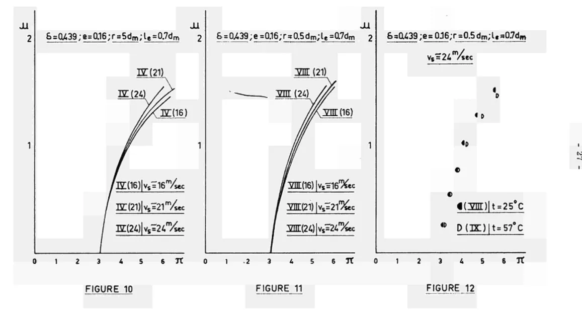
Effects of the velocity Vs in the nozzle discharge tip are shown in figure 10 and figure 11 (phases IV and VIII, respectively).

The results shown in figure 12 (phases VIII and IX) appear to indicate that the effect of temperature (density, viscosity) is negligible.

Jet pump characteristics ( 6 = O.403) for three diffe­ rent values of the eccentricity ratio e (e = 0.16, phase VII; e = 0, phase X and e = 0.35, phase XI) are shown in figure 8. It is seen from this figure that eccentricity of the nozzle does not exhibit a significant effect for small values of the eccentricity ratio (up to about e = 0.16).

High jet pump efficiency was obtained for le = 0.7 dni.

Prom figure 13 (phases X and XIII) it can be easily deter­ mined that

for 6 = O.4O3 the maximum efficiency is ? V ^ λ = 35.8,

6

ρ 5^

= 0.339 the maximum efficiency is n~\ ]_ | = 35.6,

The effect of small variations in the distance le

(between the nozzle tip and the beginning of the mixing tube) appears to be negligible. Prom figure 9 ^phases X and XII) it can be seen that for a diameter ratio o equal to O.403 even a decrease of le by about 40^ (le from 0.7 dm to 0.4 dm) does

not affect the shape of the jet pump characteristic.

The length 1^ of the mixing tube (figure 5) was 8 timt­:

­ 23

efficiency the static pressure exhibited a maximum near the outlet end of the mixing tube (figure 14); this means that with the chosen length complete mixing is attained. In a longer tube the static pressure will decrease again toward the outlet end due to frictional losses; this will result in a decrease in jet pump efficiency. It is evident, there­ fore, that for a jet pump of good performance the length lm

of the mixing tube is equal to about 8 dm.

The length l¿i of the cone­shaped diffuser (figure 5) was equal to about 10 dm; the divergence angle β was 7 .

During the first phases of the test it was found that the efficiency of the diffuser ranged from 0.80 to 0.90.

As the efficiency of a good diffuser is about 0.85 no

PHASE I Π

n i

ra:

Έ. 2 1 2XT

V I I I

I X χ XE

xn

X I I I

0.439

IÖ1

O

O

O

b 0.403

O

O

o

o

o

0.339

o

¡o

1

o

o

0.16

O

O

O

O

O

O

o

o

o

e 0 ■·-

-o

o

o

All phases : lm= 8 dm . Id = 10dm

Phases Sand IE ; Supporting plate ¡η suction sectior s 1 0.35

O

5dm

O

O

O

"o"

o

o

Γ OSdm

O

o

o

O'

o

o

o

le

0.7dm 0.4dm

o

f

o

o

o

O

O

O

O

o

o

o

o

o

1 25°C

O

O"

o

o

o

o

o

o

o

o

o

o

Phase I : Internal surfaces relative Other phases : internal surfaces smooth t 57°C

o

TABLE — 2 3 ¿ 5 6 7 8 9 10 11 12 13 FIGURE — 6 — 6,10 — 7 7,8 11,12 12 8,9,13,16 8 9 13,16

>ly rough (galvanized) (normally polished )

to

25

JU

&=0.439 ; e=0.16 ; r = 5 dm ; te = 0.7dm

v, = 2 1 % c

π

/ w.

f

nel

—

f π I s.p.

ƒ (s.p.: supporting plates F in suction section)

JU

b=0.403 ; e =0.16; le=0.7dm

7 π 6 7 7t

FIGURE 6 FIGURE 7

JU &: =0.403 ; r

vs

=0L5dm ; le

= 21 "/sec

= 0.7d m

X

_,sr

2Γ.

7 π

Ol 8=0.403 ; e = 0;r = 0.5d _m

ν

5

*2ΐ"!4

o *

° « ( Σ ) I le=0.7dm

o(XŒ)|le = 0.4dm

7 π

26 ­

I. EVALUATION Off THE THEORETICAL LOSS C0El'Vi.''ICIENT5

1.1. Evaluation of K

_m

It is a good idealization to assume that in the mixing tube the pressure loss ΔΡιη due to friction is

A* m = fm d^ · * <? va ·

m

d~ · * f

m >

where

f is a friction factor,

L is the effective length of the mixing tube, v„ is the average velocity along the wall of the

mixing tube.

If, for simplicity, it is assumed that (figure 1)

VZ + vt

va = 2 '

it follows that

m L )

The x^ressure l o s s i n t h e mixing t u b e was a l s o v/ri' o

m ·

•

'-¿f

- O V g

t- _ .,-> L / ι τ t \ *" ' m ' - m * T T V. -" + ···' v " ; .

ilo ne e

v 'm

25

-JU JU S=0l¿39;e=0.16;rg5dm;le=0.7dm 2

rg(16)|vs=16m/5<

I5ZI(21)|vs=21m/i«

3g(24)[vs=24%

JU

S=0¿39;e=0.16;r:*0.5dm;le=Q.7dm 2

UZE (21)

M (16)

m(16) |vs=16%c

2ΠΠ21) |vs=21% _sec

mL(2ü)\^=2Öi _sec

& =(H39 ;e=0J6;r=0.5dm;l«

vs = 2¿m%ec

I D

«D

©

φ

«C2nr)|t =

«D D ( I K ) | t =

a07dm

25°C

57° C

CO

- α

0 1 2 3 4 5 6 7 t 0 1 2 3 4 5 6 Tt 0 1 2 3 4 5 6 1 t

28

o(D)

-10000

-20000

-30000

"!tø

420 mr

U 6=0.403 ; JU = 1.89 «16=0.403 ;ju = 1.80 'l I !

I

(T) (X) (vj (?)

MIXING TUBE

FIGURE 14

FIGURE 13

Experimentally determined

jet" pump characteristics

29

¡/rom

f V s

+

p t (

S

m -

S

s

)

= f V

J

m

i t can be found that

v

s -

v

t

=

τς <

v

z -

v

t

)

·

"üince ν - ν, > O , it follows that

vz - vt > 0

or ^ < 1

that

'nen

A good approximation is obtained if it is assumed

Ιί = 0.5 and L = 0.75 lm .

0.75 1τη ?

¿; = f L1 (£ + }, χ 0. 5 Γ .

m m d v

m

'or a smooth internal surface of the mixing tube ir:;

1

the value of the friction factor f may be taken as 0.018

Consequently, if ­τ— = 8,

Κ = 0.018 χ 0.75 x 8 ('; + ·' χ 0 . 5 )2 =

m

­ 30

1.2. Evaluation of Kd

The efficiency η , of the diffuser (figure 1) is defined by l

(Pc +pghc

) ­ (pz +nghz

)

^d =

_{¿ p(v}

ΓΤ7Τ2 ­ΤΓ­

_{z ­ vc)} 1

*

Therefore

(p

c

+ f g h

c

) ­ (p

z

+Ç)gh

z

)

= η

ά

. ^ ( ν

2

- ν

2

) .

It was already seen that for the diffuser

P

Z

- P

C

=

­<¡>s(h

z

­ h

c

) ­ ¿p(v

2

­ v

2

) + K

d

.:

;

p

2

or

(pc +righc) ­ (pz +^ghz) = >;n(v| ­ v2) ­ Kd.;.Ç>v2

Hence

V ^

( V

Z "

V

C

} =

"T

(V

2 *

V

G

}

­

K

d'

;

'f

v

Z

or

Κ

=

_{( 1}

- v )

_i

- ( î )

Since pvnSri = p v .73m,

it follows that

C m I m \

where dQ is the diameter of the diffuser outlet

(figure 5 ) .

Therefore

K

a

= d ­ V

1 - t à

31

-If the length lci of the cone-shaped diffuser is equal to 10 dm and the divergence angle β is 7

(figure 5), then it can be readily found that

dC = dm + 2 λά t a n 2 =

= dm + 2 0 dm tan3°30' =

= (1 + 20 χ 0 . 0 6 1 2 ) dm =

Hence

= 2.22 äm

dm 1

dc - 2.22 '

The average value of the diffuser efficiency TV, was found to be about 0.85.

Consequently

V

=

(1

- 0.85)

I

1 -

[rr^l

)

32 ­

1.3. Evaluation of K

s

and K^

Prom the derived expression for the total

pressure ratio

TX

it follows that the total pressure

ratio f

or ax = 0, represented by ( ^ ^..Q , is given "by

1 + Ks

( l t

^ = °

=

2 Ó

2

­ (1

+

K

m +

K

d

) ¿ 4

Hence

As it was found that Κ = 0.06 and K, = 0.14,

it follows that

m

1 + Κ + Κ. = 1.2

_m

_d

anu

Κ

s

■

( I f

i u = o (

2

¿

2

­ 1.26+) ­ 1 .

The value of

( T T ^ ­ Q i s represented by the point

at which the jet pump characteristic curve intersects

the Tf­axis (figure 2 ) .

From tiie experimentally determined jet pump

characteristics it is readily seen that

( Τ Τ ) ^= 0 = 4.95 for 6 = 0.339 (figures 13 and 16),

( T T

iU=0

= 3

·

6 0 f o r

¿

=

° ·

4 0 3

(

fi

^

aires

?»

8

»

13 ar,d 1 6

^

(TOJU-0

=

3.05 for

8 =

0.439 (figures 6, 10 and 11).

Prom these conditions the average value for K

a

is found to be abΟ\Λt 0.05.

The loss coefficient K. may be taken equal to K

e

:

33

d . CHAHAC'fEfllüTICS AND MAXIMUM EFFICIENCY

Upon inserting the values

K

s = 0.05, Kt = 0.05, Km = 0.06 and Kd = O . H

into the derived expression for the total pressure ratio 7f,

the result is

7T =

2 ¿>4

1.05 - 1.05->u¿ S - j —

(1 - δ

2

)

2

2¿¡

2 +

^ 2

S

_ 1.05-α

2

Κπ

- 1.2(1

+JU)

2

¿>

4

1 ­ 62

(1 _ £2>2

By means of this expression theoretical characte­

ristics

(JU

as a function of 7t) were determined for

S = O.403 and ¿> = 0.339.

It can

be seen from figure 15 and figure 16 that these

characteristics agree excellently with the experimentally

foimd characteristic curves for e = 0, r = 0,5 dm,

l

e

= 0.7 dm, lm = 8 dm and Id = 10 dm (phases X and XIII).

Theoretical characteristics for other values of

6

were also found to be in good agreement with experimental

results.

Therefore, characteristics of the tested type of

jet pump can

be predicted to a high degree of accuracy by

means of the expression

Τΐ =

0+K

s

) - ( l ^ g —gg

'^

+

^

Ä -

( 1 + K

i>

2

7 ^ 2 7 - (1+VK

d

)(1

+

u,)2¿4 '

v/Vie r e

Ks = 0 . 0 5 , Kt = O.O5, Km = 0 . 0 6 and Kd = 0 . 1 4

34 ­

For each of these û values the relationship between the jet pump efficiency Tl and the mass flow ratio JU could also be calculated since ï) is defined by

V

_{TT­ 1}

The results are shown in figure 18; it is seen from this figure that the maximum efficiency is dependent upon the value of the diameter ratio 6.

In figure 19 the maximum jet pump efficiency Y]m is

given as a function of o. '

The mass flow ratio at maximum efficiency (jum) as a

function of the diameter ratio S is shown in figure 20; the total pressure ratio at maximum efficiency ( 7Tm7 as a

function of δ is also shown.

Efficiency of jet pumps

Theoretical jet pump characteristics ( Ks =0.05 ; K t =0.05 ; Km=0.06 ;Kd = 0.14)

0.35 £>:(U

0.30

0.25

0.20

0.15

0.10

0.05

fc;0.3

£>:0.25

00

- 36

T|m

0.40

0.30

0.20

0.10

o

Maximum efficiency of jet pumos (Ks = a05;Kt =0.05 ; Km = 0.06,Kd:=0:U)

0.1 0.2 03 04 0.5 0.6 0.7 0.8 09 6

FIGURE 19

6

5

4

3

2

1

0

10

15

Mass flow ratio at maximum efficiency

(Ks=0.05;Kt=0.05;Km = 0.06;Kd=Q14)

0.1 0.2 0.3 0.4 05 0.6 0.7 08 0.9 &

37

K. UST¿Ia,l.MATION OF ABSOLUTE DIMENSIONS

It was seen that in a steady state

2

a i l

or

HA­ ΗΒ=φ.­|γν2 ,

wie re

φ = d

+

K

s

)

.

(1

-

K

t ^

2 ( 1

T^p

Since the total pressure ratio 7Í is defined by

π =

HA * E3

H0 " HB

it follows that

o r

i'roi

7t(HG - HB) = φ . ^

vs =

2 1í(fip - Ho)

0 1XB'

?<P

G.

S ν = — and

s s

?

it can be readily found that

• ­ 3.14 ,2 's ~ 4 us

ds =

38 ­

Upon inserting the derived expression for ν the result is

dg = 1 . 1 3 | ^

<p

f*(

Ηπ ­ Ηχ.)

If in a system (figure 4 ) , at maximum jet pump

efficiency, the required values of the mass flov/ rates are G.. and Gp, then the value of the mass flow ratio is

V

=

τη

·

The value of the diameter ratio δ for maximum jet pump efficiency at the required value of the mass flow ratio jUni can be found from figure 20; for these values of Mm and o

the value of the total pressure ratio Tfm can also be found.

For this case the value of the coefficient φ is

(p= (1

+ K s > ­ (1 t' m

(1

ó*

TP

)

The difference in total pressure at 0 and Β (figure 4; is equal to the sum of the separate pressure losses due to friction and to changes in velocity resulting from gradual or abrupt changes in the cross­sectional area of the fluid

conduit CÏÏB; hence the pressure loss HQ ­ îîg at the required flow rates can be predicted from the surface roughness and. trie shape and size of the fluid passages of the conduit CDB.

ì'ince Ò is defined by

6

=

ΐ

m it follows that

­ 39 ­

Other d intensions can be determined from ds and dm

since for the considered type of jet pump (figure 5)

1 = 6 d . 1 = 0,7 dm , 1 = 8 dm , L· = 10 d ,

n s ' e m ' m m ' d m '

r = 0.5 dŒ ,o<= 10°­15° , β = 7°.

Example

If it is required that, at maximum jet pump

efficiency, the mass flow rates G­j and G2 are 12.2 kg/sec and 19.7 kg/sec, respectively, then the required mass flow ratio JU is

_ C2 _ I9.7 _ ,fi1

It is seen from figure 20 that for· the α ιΕ vaivi e 0^

1.61 the diameter ratio δ is 0.43; for these values of uxr,

and 0 the value of the total pressure ratio 7T is seen to be about 5.5.

i^or ja = 1.61 the coefficient (p is, if Κ = Κ, ­ 0.05,

(ρ= (1

+

κ

β

) ­

(1

­

K

t ^ m

(1

}\if

= 1.05 ­ 1.05 Χ 1.612 ° ·4 3 Λ Λ = 0.91

(1 ­ 0.43'­Γ

I f the f l u i d d e n s i t y i s taken as 750 kg/irr arid tino

2

nressure loss H~ ­ lip as 50 000 N/m , it follows xhat th diameter of the nozzle tip is

40

-d

s =

1

·

1

3 | / ^

φ

2

f V t " %)

4/

= 1 . 1 3 | Λ ^

/ 2 x 7 5 0 x 1

1

. 5 x WOO =0.0211 m =

= 2 7 . 1 mm .

The diameter of the mixing tube is

d

m =

J

= Ü7ÏI =

63

'° ™

n

'

Por the considered type of jet pump (figure 5)

1 . = 6 d , 1 = 0.7 d , 1 = 8 d , 1, = 10 d , η s ' e * m ' m m ' d η '

r = 0.5 ä , c<= 10°­15° , β = 7°. m

It follows, therefore, that

1 = 163 mm , 1 = 44 mm , 1 ­­ 504 mm , 1­, ~ 630 r.j

L i. v ? 1X1 * 1

41

L. CONCLUSIONS

a. The performance of a jet pump is dependent upon the shape of the jet pump characteristic.

b. The characteristic of a jet pump with a given diameter ratio S can be predicted by means of the equation

9

(1-fKj-(1+K

+

)ar-7t =

6*

a

"

~

TT?7

2

¿2

+2ul

2 J ^ _

(1+

K

t

)^2 _

^

_

( 1 + V

K

d

) ( 1

+

^ )

2

6

4

good agreement with experimentally found characteristics of high­performance jet pumps was obtained for

Kg = 0.05 , Kt = 0.05 , Km = 0.06 and K¿ = 0.14.

c. High jet pump performance was attained when the following conditions were satisfied (figure 5 ) :

\ = 6 ds

o< = 10°­15° e < 0 . 1 6 r = 0.5 dffi

h

= °·

7 d

m

!τη = 8 dm

m m

^ =_d 1 0 d™ _m

β

= 7°

.

­ 42 ­

d. For a given type of jet pump the maximum efficiency is dependent upon the value of the diameter ratio.

e. An efficiency in excess of 0.37 can be realized.

ACKNOÏÏLEDGEI/IENT

The author wishes to acknowledge the cooperation of E. Buur, who assisted in constructing and operating the experimental equipment, and L. van Zijl,, who pre­ pared the figures.

EFEUEN CE o

G. Flügel, "Berechnung von Strahlaîroaraten", VDI­Forschungsheft 395 Γ

Deutscher Ingenieur­Verlag, Düsseldorf

F. Schulz and K.H. Fasol, "Wasserstrahlpumpen zur Förderung 'von Flüssigkeiten" ;

Wien, Springer­Verlag, 1958.

"VDI­Durchflussmessregeln";

43

A P P E N D I X

1. Reduction of the test data

1.1. fressure losses

The difference in total pressure at two points (the pressxire loss between two points) can be deter­ mined by means of a U­tube manometer.

If a U­tube manometer is connected to static pressure taps located at X and D (figure 5), then

P

X

+ <j>g(h

x

- h

D

) + ^ g E

X D

=

P l )

+ r ^ g E

0

,

whe re

Py is the static pressure at X, p­ß is the static pressure at D, ρ is the density of the fluid,

is the density of the manometer fluid,

g is the acceleration due to gravity, hY is the height of X above the reference

Λ level 0­0,

h­p. is the height of D above the reference

v level 0­0,

Ey­p. is the manometer deflection.

Hence

Ρχ ­ P D + ^ h x ­ hD> = % ' ^ e ^ C D ·

If v¿ and VT) are the fluid velocities at A and D, respectively, the total pressure Η­v at X i.

­ 44 ­

and the total pressure Ηη at D is

HD = PD + pgh-Q + ¿^v2 .

Therefore, the pressure loss between X and D is

II _X

_-

_H

_{D = PX * PD}

₊

_^

_h

_X

_'

_h

_D

_{} +}

_ψ

_ν

_Χ

_'

_V

_D

_}

₌

=

% '

f)ft])

+

*Y

V

1 -

V

D

}

'

The difference in total pressure at two points

(the pressure loss between two points) can also be

calculated from the readings of two­ separate pressure

gauges.

If a jiressure gauge M^ is connected to a

pressure tap located at A and a pressure gauge iij, is

connected to a pressure tap located at D (figure 5 ) ,

then

E

A * B

D = PA + ^

h

A » h

H A

) ­ {

PD + f ^

h

D " * W } <

where

E. is the reading of the pre?­sure gauge I.L ,

Ej. is the reading of the pressure gauge KL·,

ρ« is the static pressure at A,

h» is the height of A above the reference

A

level 0­0,

hjyrA is the height of the pressure gauge I.I»

above the reference level 0­0,

^MD ^

S

^^

e n e

i S

n

^ °f

'the

pressure gauge

L­­,

above the reference level 0­0.

Hence

45

if

v^ is the fluid velocity at A, H. is the total pressure at A, Hy. is the total pressure at D,

then the pressure loss between A and D is

HA - HD = pA - pD + <^g(hA - hD) + f^(v2 - v2) =

­ 46 ­

1.2. ft"as3 flow rates

Orifice plates 0­| and O2 (figure 3) were used tó determine the mass flow rates G.. and G.. + Gp, respectively (figures 1 and 4 ) .

If

ΔΡ­j is the static pressure drop across the orifice plate 0..,

ΔΡρ is the static pressure drop across the orifice plate 0?,

then the mass flow rates G1 and G.. + G0 are given by

7j 2

G1 = C*01 · 4 d0 1

G-I + G2 = O^ 0 2 · 4 d0 2

m

Δ ρ .

ñ

2 Ο Δ Ρ _{2 1} where

ο<"01 ando^Qp are flow coefficients for the orifice

plates 01 and 0?, respectively,

dQ1 and dQp are the diameters of the orifices in

the plates 0. and 0?, respectively.

If U­tube manometers are used to determine the static pressure'differences across the orifice plates 0. and Op, then

ΔΡ 1 = (<¡m ­ f ^Ε0 1 .

ΔΡ2 = ( < ¡ m ­ ^ SE0 2 ■

47

-Hence

G1 = C* 0 1 · 4 d0 1

/

₂

^ m " ^ S |/^θΤ .

G1 + G2 = c ^0 2. ^ d0 2

/

48

1.3. The mass flow ratio

The mass flow ratio

JU

is defined by

Go

JU =

*7 '

It was already found that

G

1

+ G

?

= 0 ^ 2 .

j

d

02

'

2

^m

-

V

)S

|/í¡

J0 2 »

π o

G

1

_C

*O1 ·

4

a

01

w„

-

-0).

ν

Hence

ax

=

_*7

G2

=

°*Ό2

°^01 · G1

TT ' 4

TT 4

+ (

ö1

, 2

d0 2

, 2

d01

' 2 - 1 =

|/

2

^Vm

N

(

r*

- ? ) s /"s

0 2

- P ) g / 201

­ 1

or

ΟΛ

=

°^02

,d

02

o ^

r

d

01

E

S

02

01

49

1.4. Velocities

The fluid velocity vs in the discharge tip of

the driving nozzle (figures 1 and 5) is

vs =

S G. m 1

f .

a

a ?

_m

d

mf

S

1

1 G1

f o ¿

2

V

m where

G1 is the mass flow rate in the driving nozzle,

d„ and d„ are the diameters of the nozzle tip .Q τηm and the mixing tube, respectively, *?

S and S are the flow areas of the nozzle tip

α m and the mixing tube, respectively, τη

*-Ò is the diameter ratio, defined by

k - s

m

It was already found that

G1 = °\)1 · 4 d01

/

₂

^ - ^ e | / V i

it follows, therefore, that

=

-gÇ-fcoí

· Î

d

01 |/

2

^m-^S

^

The velocity v% at the outlet end of the mixing tube (figure 5) is

VZ =

u1 + '"2

-ψτ

where G9 is the mass flow rate in the suction section

50

-Hence

G

VZ = ( 1 +OA) - g - 1 _r ,

'm

where -u i s the mass flov/ r a t i o , defined by

G2

If

then

3, is the cross­sectional area upstream from the driving nozzle at A,

S.Q is the flow area in the suction section

*

a t B,

S

n

i s the flow a r e a a t t h e d i f f u s e r o u t l e t

υ

a t C,

G.

G.

ν

-

1

- I L . ÍS

ί , J U G Λ G

2 _ ^ u 1 _ , 1 m

ψί~ψί~ Fm^ '

G1 + &2 <1 + ^ G 1 M ^ G1 Gm

Vr = —pr* = n* = ( ! +JU) TTT- τ ~

C

f °C f

b

C f m

J

G

G

1 C2

ionsequently, since r^V- =

Ò v

g

,

\ ' m

v

z

= (1

+^)ί\

, v

A

= ^ 6

2

v

s Λ

­ 51 ­

1.5. The total pressure ratio

The total pressure ratio 7T is defined by

­r HA ­ HB

where (figures 1 and 5)

HA is the total pressure in the plane A,

Η­p, is the total pressure in the plane B, H,, is the total pressure in the plane C.

The ratio TX may also be written as

C­A « HD> ­ <H3 ­ HD>

π =

(

H

c -

!i

û) -

(FB

-

H D )

where H~. is the total pressure at D.

To determine the difference in total pressure at A and D separate spring­type gauges î... and lay. ­were used (figures 3 and 5 ) .

The difference in total pressure at G and D and. the difference in total pressiire at 3 and D were

52

-Hence

(HA - Hg) - (HB - Ηυ)

* ■ DÇ - ν - Ufe - ν

{E

A

-E

p

^

s

(h

tiA

-h

m

)

+

y(v|-v

2

)} - {(p

m

-p)gE

BI)

^p(v|-v

2

)}

2- v2)

_ W f S <hjjA-ht,],)- ( f

m

- 9)gE

B

^ìP(v¿- > _,

wnere

E, and ET. are the readings of the pressure

^ gauges M. and H­, respectively,

E­n­p. is the deflection of the U­tube manometer which is connected to pressure taps located at Β and D,

Erj. is the deflection of the U­tube manometer

which is connected to pressure taps located at C and D,

h­MA is the height of the pressure gauge KA

above the reference level 0­0,

hjwr­pv is the height of the pressure­ gauge M­p above the reference level 0­0,

vA is the fluid velocity at A,

Vg is the fluid velocity at B,

vc is the fluid velocity at C,

v­Q is the fluid velocity at D.

53

-ΛΛ = ° \ ) 2 * d_¿Γ" 0 ? °^01 · d0 1

'02

^07

- 1

- rá-|*bi · ï «ai R w ^ J T ^ l ^

"m f2

V

A = τι

6 v

s ι

m r2 v^ = -tr-JU 6 ν

xS o^-. S '

vc = ^ £ ( 1 +o i ) o2vs ,

ir =

E

A

- E

D

4

<?

g(h

MA

- h

M S

) - ( f e - f ) g E

+

y(vf

"

^m - ^S(

E

CD - * W

+

ψ

ν

0 -

V

B>

54

1.6. Significant data

a. Orifice plates (figure 3) Flow coefficient for

orifice plate 0.. Flow coefficient for

orifice plate Op

Diameter of orifice in plate 0..

Diameter of orifice in plate Op

©¿0 1 = 0 . 6 5 6

e ¿0 2 = 0 . 6 4 9

­3

d01 = 48.95 x 10~J m

d0 2 = 83.26 χ 10~3 m

b. U­tube manometers (figure 3) Density of manometer fluid

(mercury) : O

(Acceleration due to gravity: g

= 13600 kg/m3

= 9.81 m/sec1­)

c. Jet pump (figures 1. 3 and 5) Diameter of mixing tube Flow area at Ζ

Flow area at A Flow area at Β Flow area at C

dm = 60.1 χ 10""3 m

Sz = 28.4 x 10"4 m2

SA = 19.6 χ 10"4 m2

JB = 1 1 2 χ 10~ 4 m2

= 1 4 0 χ 10"4 m2

d. Pressure gauges (figures 3 and 5) Vertical distance between

pressure gauges M. and M­p

_h

MA ­ hjjjj = 0.9' m

55

PHASE I

fe = 0 . 4 3 9 e = 0 . 1 6 r » 5 dp

h

= ° ·

7 d

m

\ ' 8 dm

t o C 25 25 25 25 25 25 25 25

Eo j

cm Hg 3 5 . 8 3 5 . 8 3 5 . 8 3 5 . 9 3 4 . 7 3 4 . 9 3 6 . 7 3 7 . 4

E 02 cm Hg

4 . 4 5 . 5 7 . 9 9 . 9 1 2 . 7 1 6 . 7 2C.8 2 7 . 9

EA - ;E0

N / 2 /nrr 199072 199206 199520 199606 189262 191224 193273 137967 EÇP cm Hg 6 0 . 6 5 8 . 3 5 4 . 9 5 1 . 4 4 3 . 2 3 8 . 7 3 5 . 5 2 4 . 6

E BD cm Hg

0 0 - 0 . 4 - 0 . 9 - 2 . 1 - 3 . 1 - 4 . 5 - 7 . 3

vs

m / /sec 2 1 . 4 2 1 . 4 2 1 . 4 2 1 . 4 2 1 . 1 2 1 . 1 ? 1 . 7 2 1 . 8

JU

0 . 0 1 0 . 1 2 0 . 3 5 0 . 5 1 C.74 0 . 9 8 1.16 1.48

Έ

2 . 9 9

3 . 1 0

3 . 2 9

3 . 4 7

3 . 8 5

4 . 2 2

4 . 5 0

5 . 6 0

FIGURE

6

TABLE 2

PHASE M

fe = 0 . 3 3 9

G = 0 . 1 6

r - 5 dm

1n "_{6 in} ° ·7 dm

\ « 8 dm 1d - 1 0 dm

t O C 25 25 25 25 25 25 25 25 25 25 25 25 25 25 25 25 25 25 25 25 25 25 25 25 Eoi cm Hg

8 . 1 8 . 1 8 . 2 8 . 2 8 . 3 8 . 3 8 . 5 8 . 6 1 5 . 3 1 5 . 3 1 5 . 3 1 5 . 4 1 5 . 5 1 5 . 8 1 6 . 0 1 6 . 1 2 0 . 0 2 0 . ) 2 0 . 0 2 0 . 1 2 0 . 4 2 0 . ' 2 0 . 6 2 1 . 0

Eo2

cm Hg

1.1 1.6 2 . 9 4 . 3 5 . 8 7 . 1 9 . 0 1 1 . 2 1.9 3 . 2 5 . 4 7 . 9 9 . 4 1 4 . 5 1 ? . 9 2 2 . 9 2 . 9 5 . 0 6 . 5 1 1 . 2 1 4 . 9 2 0 . 3 2 5 . 8 2 9 . 9

EA- ED

N / 2 / m '

147079 147079 146098 145117 145117 145117 143155 142174 278800 277819 273086 277105 276391 274696 274386 272286 358975 357013 357013 351127 3^1127 3 " 1 1 2 7 3511 r? 351127

ECD

cm Hg

2 5 . 6 ! 2 4 . 7

2 2 . 5 2 0 . 7 1 8 . 6 1 6 . 8 1 4 . 5 1 1 . 6 ' 4 8 . 3

4 5 . 7 4 2 . 5 3 9 . 4 3 7 . 5 3 1 . 8 2 6 . 7 2 2 . 4 6 1 . 9 5 8 . 3 5 6 . 2 5 0 . 2 4 5 . 3 3 9 . 2 3 2 . 0 2 6 . 8

EBD

cm Hg

0 0 - 0 . 4 - 0 . 9 - 1.6 - 2 . 2 - 3 . 2 - 4 . 2

0 - 0 . 1 - 0 . 5 - 1.2 - 1.7 - 3 . 5 - 5 . 2 - 6 . 8

0 - 0 . 4 - 0 . 7 - 2 . 3 - 4 . 8 - 6 . 1 - 8 . 7 - 1 0 . 9

vs m /

/sec

1 6 . 8 1 6 . 8 1 6 . 9 1 6 . 9 1 7 . 1 1 7 . 1 1 7 . 3 1 7 . 4 2 3 . 2 2 3 . 2 2 3 . 2 2 3 . 2 2 3 . 3 2 3 . 5 2 3 . 7 2 3 . 8 2 6 . 4 2 6 . 4 2 6 . 4 2 6 . 5 2 6 . 7 2 6 . 6 2 7 . 0 2 7 . 1

JU

0 . 0 5 0 . 2 7 0 . 7 1 1.08 1.39 1.66 1.96 2 . 2 6

r 0 . 0 1

0 . 3 1 0 . 7 1 1.06 1.23 1.74 2 . 1 2 2 . 4 2 0 . 0 9 0 . 4 4 0.64 1.14 1.45 1.85 2.2C 2.45 îf

5 . 0 3 5 . 2 1 5 . 6 0 5 . 9 3 6 . 3 7 6 . 8 0 7 . 2 7 ; 8 . 1 6 ^ 4 . 9 4 5 . 1 7 5 . 5 1 5 . 8 5 6 . 0 6 6 . 7 3 7 . 4 7 8 . 1 6 4 . 9 1 5 . 1 9 5 . 3 5 5 . 7 1 6 . 0 4 6 . 7 0 7 . 5 2 8 . 1 7

FIGURE

56

-PHASE I g

fe « 0 . 4 3 9 e = 0 . 1 6

r - 5 d Q

m m

1 β 10 d

α m

t 0 C 25 25 25 25 25 25 25 25 25 25 25 25 25 25 25 25 25 25 25 25 25 25 25 25

EPJ EQ2

cm Hg cm Hg

2 0 . 2 2.5 2 0 . 2 3.3 2 0 . 2 4 . 1 2 0 . 2 5 . 1 2 0 . 2 6 . 7 2 0 . 4 8 . 3 2 0 . 8 10.3 2 1 . 0 12.7 2 1 . 2 1 4 . 7 3 4 . 2 4 . 9 3 4 . 2 6 . 0 3 4 . 2 7 . 5 3 4 . 3 9 . 3 3 4 . 4 11.7 3 4 . 6 1 3 . 7 3 4 . 8 1 6 . 0 3 5 . 1 2 0 . 1 3 5 . 4 2 5 . 1 4 3 . 2 6 . 0 4 3 . 0 10.4 4 3 . 3 15.7 4 3 . 7 19.7 4 4 . 2 25.9 4 4 . 7 3 3 . 6

E A - J D

k * /

N / 2 ' m 111230 111230 111230 111230 110249 110249 108518 108518 103613 189441 191403 190422 189441 187479 186498 185654 181730 177090 238491 237510 235548 232605 225875 220833 EP° cmHg 34.1 32.6 31.2 29.6 27.0 24.4 21.6 17.5 13.5 55.8 54.5 52.1 49.0 45.2 42.4 38.6 31.7 22.8 70.4 63.4 55.5 49.0 38.3 28.7

τ ■ " " ■ '

-cm Hg

0 0 - 0 . 1 - 0 . 3 - 0 . 8 - 1.2 - 1.9 - 2 . 7 - 3.5

0 - 0 . 1 - 0 . 3 - 0.8 - 1.4 - 2 . 0 - 2 . 6 - 4 . 0 - 6 . 0 - 0 . 1 - 0 . 7 - 2 . 0 - 3 . 2 - 5 . 4 - 7 . 7

vs

JU m /

/sec

1 6 . 1 0 . 0 1 16.1 0 . 1 6 1 6 . 1 O.29 1 6 . 1 0 . 4 4

16.1 0.65

1 6 . 2 0.83

16.3 1.02

16.4 1.23

16.5 1.39

20.9 0 . 0 8

20.9 0.20

20.9 0.34

21.0 0.49

2 1 . 0 0.67 21.0 0 . 3 0 2 1 . 1 0.95 2 1 . 2 1.18 2 1 . 2 1.41

2 3 . 6 0 . 0 6 23.5 0 . 4 1 2 3 . 6 0.73 23.7 0 . 9 2

23.8 1.20

23.9 1.48

π

3 . 0 2 3.16 3 . 2 9 3.48 3.69 Λ.03 4 . 4 2 5 . 1 9 5.95 3 . 0 9 3.19 3 . 3 2 3.48 3.70 3.84 4 . 1 7 4 . 7 6 5 . 8 1

3.05 3.35 3.73 4 . 0 9 4 . 8 0 5 . 7 1

FIGURE

10

6,10

10

TABLE 4

PHASE Y

fe - 0 . 3 3 9 e « 0 . 1 6

* - 5 dm 1 - - ° · 7_β dm _IQ 1 * - 8 dm

m m

1 m 10 dm

α m

t 0 C 25 25 25 25 25 25 25 25 25 25 25 25 25 25 25 25 Eoi

cm Hg

1 4 . 2 1 4 . 2 14.3 14.5 14.5 1 4 . 7 14.9 1 5 . 0 2 1 . 6 2 1 . 5 2 1 . 6 2 1 . Π 2 2 . 0 2 2 . 2 2 2 . 4 22.5

Eo2

cm Hg

1.8 2.5 5 . 1 G.8 11.0 14.3 17.5 20.3 2 . 8 5 . 1 8 . 0 11.9 16.3

22.6

26.5 3 0 . 4

E A - ED

N / 2 / m ' 258513 255570 260930 257213 257748 257042 256061 256453 387603 387868 387868 388142 396255 379264 379529 379529 Eco cm Hg 44.9 42.4 39.4 34.7

: 3 2 . 0

27.8 23.1 19.2 67.6 63.1 59.2 5 4 . 2 48.7 40.4 34.7 29f3

E B D

cm H g

0 - 0 . 1 - 0 . 5 - 1.7 - 2.5 - 3 . 7 - 5 . 0 - * , 1

0 - 0 . 1 - 1.0 - 2 . 2 - 3 . 6 - 6 . 0 - 7 . 7 - 9 . 4

vs

m / /sec

22.3 22.3 2 2 . 4 22.6 2 2 . 6 2 2 . 7 2 2 . 9 2 2 . 9 27.5 27.5 27.5 2 7 . 6 2 7 . 7 2 7 . 8 2 8 . 0 2 8 . 1

JJ

0 . 0 2 0.23 0 . 7 1 1.23 1.50 1.83 2 . 1 1 2.34 0.03 0 . 3 9 0.74 1.12 1.47 1.90 2.13 2 . 3 4

π

4.95 5 . 1 9 5 . 5 4 6 . 1 2 6.49 7 . 0 7 7 . 9 3 8.Q5 4.87 5 . 2 0 5 . 4 7 5 . 8 6 6.32 7.03 7.73 8 . 5 1

FIGURE

57

-PHASE 2 1

fe » 0 . 4 0 3 e = 0 . 1 6

r - 5 dm

\

-

° ·

7 d

m

^ - 8 dm

! d » 1 0 dm

t o C 25 25 25 25 25 25 25 25 Eoi cm Hg

2 2 . 8 2 2 . 8 2 2 . 8 2 3 . 0 2 3 . 1 2 3 . 4 2 3 . 7 2 3 . 9

E 02 cm Hg

3 . 0 3 . 4 4 . 8 7 . 0 1 0 . 0 1 3 . 6 1 7 . 2 2 1 . 7

EA- E0

N / 2 / m ' 1 9 4 1 6 7 196129 196129 1 9 4 1 6 7 1 9 2 4 7 2 190510 1 8 7 5 6 7 184665

Eco c m H g

4 7 . 8 4 6 . 5 4 4 . 9 4 1 . 5 3 7 . 2 3 2 . 4 2 6 . 9 2 0 . 0

EßD cm Hg

0 0 - 0 . 2 - 0 . 6 - 1.5 - 2 . 5 - 3 . 9 - 5 . 6

vs

m / /sec 2 0 . 1 2 0 . 1 2 0 . 1 2 0 . 2 2 0 . 2 2 0 . 4 2 0 . 5 2 0 . 6

JU

0 . 0 4 0 . 1 1 0 . 3 2 0 . 5 8 0 . 8 9 1.20 1.45 1.74

Tf

3 . 6 6 3 . 7 7 3 . 8 6 4 . 1 0 4 . 4 5 4 . 9 1 5 . 5 4 6 . 6 2

FJGURE

7

TABLE 6

PHASE SK

fe = O . 4 0 3 e = 0 . 1 6 r = 0 . 5 dm

m

* · =

° ·7 d

m

1 = 8 dm

m m

1 , » _α 10 d _m t 0 C 25 25 25 25 25 25 25 25 Eoi cm Hg

2 3 . 3 2 3 . 4 2 3 . 4 2 3 . 6 2 3 . 7 2 3 . 7 2 3 . 8 2 3 . 9

E02 c m Hg

3 . 1 4 . 3 6 . 7 9 . 7 1 2 . 7 1 5 . 1 1 9 . 3 2 3 . 4

EA- ED

N / 2 / m * 202149 201168 2 0 0 1 8 7 2 0 0 1 8 7 199206 199206 197244 196263

EC D

cm Hg 4 9 . 6 4 7 . 0 4 3 . 3 3 8 . 9 3 5 . 0 3 0 . 5 2 5 . 6 2 0 . 8

E BD cm Hg

0 0 - 0 . 6 - 1 . 4 - 2 . 4 - 3 . 8 - 5 . 3 - 6 . 8

vs

m / /sec 2 0 . 3 2 0 . 3 2 0 . 3 2 0 . 4 2 0 . 5 2 0 . 5 2 0 . 6 2 0 . 6

JU

0 . 0 5 0 . 2 3 ; o . 5 3 0 . 8 4 1.10 1 . 3 6 1 . 6 2 1 . 8 4

TT

3 . 6 1 3 . 7 9 4 . 0 4 4 . 4 2 4 . 7 7 5 . 2 4 5 . 8 1 6 . 5 2

FIGURE

7,8

58

-PHASE TUT

fe = 0 . 4 3 9 e = 0 . 1 6

r = 0.5 df f i

Xe " ° ·7 dm

1 = 8 d

xm ° am 1 * « 1 0 dm

a m t C 25 25 25 25 25 25 25 25 25 25 25 25 25 25 25 ' 25 25 25 25 25 25 Eoi

cm Hg

20.5 2 0 . 5 20,5 2 0 . 6 2 0 . 7 2 0 . 7 2 0 . 9 2 1 . 0

3 4 . 7 3 4 . 7 3 4 . 7 3 4 . 9 3 5 . 0 3 5 . 2 3 5 . 2 A4.3 4 4 . 3 44.4 4 4 . 4 44.5 4 4 . 7

Eo2

cm Hg

2.8 3 . 9 5 . 3 7 . 1 9 . 1 1 1 . 1 13.5 1 6 . 0

5 . 1 7 . 7 11.3 1 4 . 7 18.3 2 2 . 4 2 7 . 1 8 . 6 12.7 1 7 . 0 2 2 . 0 2 8 . 0 3 4 . 1

E A - ED

N / 2 / r r r

113992 113992 113011 113278 112297 112564 110602 110602 193453 192472 192472 191758 190062 189617 137871 2¿34c>4

243384 2438Γ4 240227 238667 237108 Eco cmHg 34.5 32.1 29.8 27.2 24.4 21.6 18.4 15.0 57.5 52.5 47.0 42.5 37.3 31.7 25.3 68.9 62.5 56.4 49.0 40.6 31.8 E BD

cm Hg

0 0 - 0 . 3 - 0 . 7 - 1.2 - 1.8 - 2.5 - 3 . 1

0 - 0 . 4 - 1.0 - 1.8 - 2.8 - 4 . 1 - 5 . 7 - 0 . 1 - 0.8 - 1.8 - 3 . 4 - 5.3 - 7 . 4

vs

m / /sec

16.2 1 6 . 2 16.2 16.2 16.3 16.3 16.4 16.4 2 1 . 1 2 1 . 1 21.1 2 1 . 1 2 1 . 2 2 1 . 2 2 1 . 2 23.8 23.8 23.8 23.8 23.8 2 3 . 9

JU

0.06 0.25 0.45 0.68 0 . 9 0 1.10 1.30 1.50 0 . 1 0 Ü.35 0.64 0.35 1.08 1.28 1.52 0.26 0.54 0.77 1.02 1.28 1.51

π

3.08 3 . 3 1 3.51 3.80 4.15 4 . 5 6 5.13 5.86 3.07 3.33 3.68 3.96 4 . 4 1 4 . 9 1 5.67 3.19 3.49 3.31 4.19 4.79 5 . 6 1

FIGURE

11

11

11,12

TABLE 8

PHASE I X

fe = 0 . 4 3 9 e m 0 . 1 6

r = 0 . 5 dm

Xe " ° ·7 dm

1 = 8 d

m m

t

"c

57 57 57 57 57 57

E01 E02 !

cm Hg cm Hg

4 4 . 3 8.5

1

4 4 . 3 12.7 ,

4 4 . 5 ; 17.0

4 4 . 5 2 1 . 9 !

4 4 . 7 2 8 . 0

4 4 . 7 ; 3 2 . 6 j

E A- E D ¡ Eco

/ m2 cmHg

239960 6 8 . 8

239960 6 1 . 9

239113 i 5 5 . 3

2374I8 4 8 . 0

234606 3 8 . 1

230947 . 3 0 . 1

TAI 3LE 9

EBD

cm Hg

0

- 0 . 8

- 1.9

- 3 . 4

- 5.5

- 7 . 4 vs

m / /sec;

23.9

2 3 . 9 ;

2 4 . 0 !

2 4 . 0 ''

2 4 . 1

2 4 . 1 j JU

0 . 2 6

0 . 5 4

0 . 7 7

1.01

1.27

1.46

π

3.16

3 . 4 7

3 . 8 1

4 . 2 4

4 . 9 7

5.65

FIGURE