The Exchange Rate and US Tourism Balance of Trade

Munich Personal RePEc Archive

The Exchange Rate and US Tourism

Balance of Trade

Cheng, Ka Ming and Kim, Hyeongwoo and Thompson,

Henry

Auburn University

October 2009

Online at

https://mpra.ub.uni-muenchen.de/18318/

The Exchange Rate and US Tourism Balance of Trade

Ka Ming Cheng

Hyeongwoo Kim

Henry Thompson

Auburn University

October 2009

This paper investigates evidence on the effect of dollar depreciation on the US tourism balance

of trade. Export revenue and import spending functions are estimated separately with structural

vector autoregressive methods to better capture the dynamic adjustment to exchange rate shocks.

Quarterly data cover the period of floating exchange rates from 1973 through 2007. Depreciation

raises long term US export revenue but there is no effect on import spending.

JEL: C32, F10

Keywords: balance of trade, exchange rate, tourism, structural vector autoregressive model, J-curve

The Exchange Rate and US Tourism Balance of Trade

Tourism is a growing component of the US balance of trade. The present paper separates

tourism export revenue and import spending to analyze adjustments to the dollar exchange rate.

The structural vector autoregressive model examines quarterly data during the floating exchange

rate period from 1973 through 2007.

International tourism has grown over the last three decades and has become a major

source of income for a number of countries. The US has had a trade surplus in tourism since the

1990s and tourism receipts accounted for 5% of export revenue in 2007. Worldwide, the US

ranks first in export revenue and second in import spending (UNWTO, 2008).

The balance of trade following depreciations may exhibit J-curve adjustments, first

falling due to set contracts but then rising over time. Empirical results in the J-curve literature

are mixed. Studies have investigated the J-curve with disaggregated industrial trade data but

none have explicitly examined tourism.

The following section discusses the theoretical framework with tourism spending a

function of income and the exchange rate, followed by a brief review of the J-curve literature

focused on disaggregated data. The third section presents the econometric model followed by

sections discussing results and concluding.

1. Tourism Balance of trade

Socher (1986) points out that tourism as a trading service had not been explicitly

integrated into trade theory but this has been recently done by Hazari and Ng (1993), Hazari

(1995), Hazari and Nowak (2003), and Hazari and Sgro (2004). The main distinction of tourism

relative to other traded products is that importers have to visit the exporting country.

Tourism is a luxury good with income elasticity exceeding one in the literature that

Dupont, Ghandi, and Weiss (2008) in a long term study of US tourism imports covering 1820 to

2000.

Vogt (2008) separates US tourism exports and imports with data from 1973 to 2002.

Error correction models on annual data find that US tourists are more sensitive to the exchange

rate while foreign tourists to the US are more sensitive to income. The present study focuses on

adjustment patterns in quarterly data and results differ. Specifically, foreign tourists to the US

are more sensitive to the exchange rate and US tourists more sensitive to income in the present

structuralvector autoregressive method.

International and domestic tourism are imperfect substitutes especially for cultural and

natural resource attractions. The assumption of imperfect substitutes follows the literature

including Rhomberg (1973), Magee (1975) Goldstein and Khan (1985), and Rose and Yellen

(1989). Consumers choose between international and domestic tourism according to preferences

and constrained by income Y.

Dollar depreciation, an increase in the price E of foreign currency, raises the foreign

tourism price in US dollars and lowers the US tourism price in foreign currency. Domestic

demand Dm for tourism abroad and foreign demand Dm* for tourism in the US also depend on

respective incomes.

Demand functions in general functional form are + + - + - +

Dm = Dm(Y, p, Ep*) and Dm* = Dm*(Y*, p/E, p*). (1)

where Y is US income, Y* foreign income, p the price of tourism in US, and p* the price of

tourism abroad. Positive cross price effects reflect imperfect substitutes. Dollar depreciation

lowers US demand Dm for tourism abroad and raises foreign demand Dm* for tourism in the US.

Supplies of US and foreign tourism Sx and Sx* are positive functions of price

+ +

Equilibrium quantities of international tourism are determined in the markets where Dm = Sx* and

Dm* = Sx. The present analysis does not include p and p* explicitly given the lack of data on

prices tourists pay but prices are implicitly included in export revenue X and import spending M.

Export revenue for the home country is X = pqx where qx is tourism quantity,

+ +

X = X(Y*, E). (3)

Dollar depreciation lowers the tourism price in the US, increasing the quantity qx and export

revenue X.

Similarly, import spending by the home country is M = Ep*qm reducing to

+ ?

M = M(Y, E). (4)

Depreciation raises the price Ep* of foreign tourism, lowers the quantity qm, and lowers import

spending M if import demand is elastic.

Separate export revenue and import spending are estimated in log linear form as

lnX = a0 + a1lnY* + a2lnE+ ε (5)

lnM = b0 + b1lnY + b2lnE + ν. (6)

If the Marshall-Lerner condition holds, depreciation raises the balance of trade. The sum of

absolute values of elasticities of export and import demands must exceed unity, |ηx|(X/M) + |ηm|

> 1 where ηx and ηm are elasticities of export and import demands. The Appendix shows the

coefficients in (5) and (6) are related to these elasticities as a2 = -ηx and b2 = ηm + 1.

The effect of depreciation on the balance of trade is also examined and the literature

includes various measures. Volume indices are examined by Goldstein and Khan (1978) and

Rosenweig and Koch (1988) and real export revenue and import spending by Houthakker and

Magee (1969), Senhadji (1998a), and Senhadji and Montenegro (1999). The difference between

Bahmani-Oskoosee and Malixi (1992) and the ratio of net exports to national income B/Y by Demirden

and Pastine (1995) and Senhadji (1998b).

Haynes and Stone (1982) propose the ratio X/M as utilized by Bahmani-Oskoosee and

Brooks (1999), Boyd, Caporale and Smith (2001), and Onafowora (2003). The present model

also utilizes B = X/M or in natural logs,

lnB = lnX – lnM. (7)

Substitute (5) and (6) into (7) to find

lnB = (a0 – b0) + a1lnY* – b1lnY + (a2 – b2)lnE + (ε – ν) (8)

or more simply

lnB = c0 + c1lnY* – c2lnY + c3lnE + μ. (9)

The J-curve effect is the hypothesis that the balance of trade falls immediately following

a depreciation due to previously arranged contracts but rises after an adjustment lag as developed

by Magee (1973) and Junz and Rhomberg (1973). The J-curve literature is reviewed by

Bahmani-Oskooee and Ratha (2004). Methodology has developed over the years but empirical

results remain mixed.

Some studies investigate sector specific responses to depreciation. Meade (1988) finds

no J-curve adjustment for non-oil industrial supplies, capital goods excluding automobiles, and

consumer goods. Doroodian, Jung and Boyd (1999) report a J-curve effect for agriculture but

not manufacturing. Yazici (2006) finds an S-curve for the balance of trade in Turkish agriculture,

rising initially before falling and finally increasing. Ardalani and Bahmani-Oskooee (2007) use

export and import data for 66 US industries and find the J-curve for only six in an error

correction model. Goldstein and Khan (1985) point out that aggregation across different

products may result in biased estimates and certainly could disguise different underlying

The present paper investigates the balance of trade in tourism including short and long

term dynamics with a structural vector autoregression SVAR and impulse response functions.

Tourism is a small fraction of international transactions and its contemporaneous effect on the

exchange rate is negligible. Though foreign income may affect the exchange rate, its short term

effect would be negligible since tourists must plan ahead for international travel and restrictions

are imposed in the SVAR model based on prior knowledge.

2. The Econometric Model

Consider the structural vector autoregressive SVAR process of integrated variables

t t t B L y u

Ay = ( ) ₋₁+ , (10)

where A is an m×m square matrix, yt is an m×1 vector of m difference stationary variables,

) (L

B is a matrix lag polynomial, and u_t is m×1 vector of m structural shocks. Shocks have

zero means, unit variance, and are mutually independent,

0 u_t =

E and Eu_tu'_t =I, (11)

where 0 is an m×1 null vector and I is an m×m identity matrix.

The structural form system of (10) is represented by the following reduced form system

of equations,

t t t C L y ε

y = ( ) ₋₁+ , (12)

where

) ( )

(L DB L

C = , ε_t =Du_t, and D=A−1. (13)

Combining (12) and (13),

Σ

DD D u Du

ε

ε ' = ' = ' =

'

t t t

t E

E (14)

Just identifying the system requires m(m−1)/2 identifying assumptions. We employ the

conventional approach proposed by Sims (1980) and utilize the Choleski decomposition of Σ to

find D, an approach that can be useful given prior knowledge on short term relations between

variables of interest.

Given the least squares estimates C(L) and Σ from the reduced form, the structural form

VAR is recovered with the identified contemporaneous matrix D followed by the impulse

response analysis for structural shocks to the system.

3. Tourism Balance of trade Results

Data on tourism export revenue and import spending including travel and air fare are

from the International Transactions Accounts of the Bureau of Economic Analysis. The nominal

exchange rate index is the Federal Reserve nominal major currencies index, a trade weighted

index including the euro, Canadian dollar, yen, pound, Swiss franc, Australian dollar, and

Swedish krona.

US income is nominal GDP. Foreign income in the rest of the world ROW income is the

sum of the nominal GDP of the five major tourist arrival countries, the UK, Canada, Japan,

France, and Germany, essentially the countries in the major currencies index. Their nominal

GDPs are from the International Financial Statistics of International Monetary Fund. Quarterly

data run from 1973 through 2007, the floating exchange rate era.

Tourism spending, revenue, and income could be deflated by the price indices but the

aggregation bias could result in unreliable estimates as discussed by Goldstein and Khan (1985).

The real exchange rate would introduce similar issues and the focus of the present paper remains

Stationarity is pretested to check whether variables are stationary converging to steady

state levels. Results of the unit root test from conventional augmented Dickey-Fuller ADF tests

are in Table 1. The number of lags is chosen by the Schwarz Information Criterion BIC.

*Table 1*

The ADF test with an intercept fails to reject the null hypothesis of a unit root for all level

variables except US income Y. The ADF test does not reject the null hypothesis of a unit root

for all level variables with an intercept and time trend. With lags added to US income, the ADF

test fails to reject the unit root null hypothesis. The Y series do not appear stationary in Figure 1.

*Figure 1*

ADF tests reject the unit root null hypothesis for all differenced variables. All variables

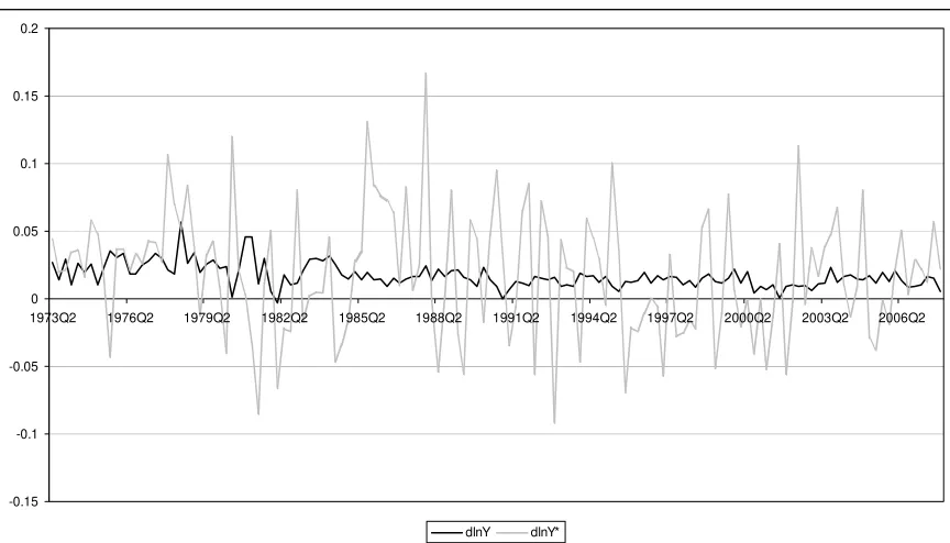
are integrated in the first order, and differences in Figure 2 and 3 appear stationary.

*Figure 2*Figure 3*

All variables are I(1) and first differencing can remove nonstationarity. An SVAR with

differenced variables provides estimates and for comparison the tourism balance of trade model

is also reported.

Contemporaneous relations of each innovation and one unit structural shocks are derived

from the estimates. Diagonal element estimates are normalized to one with Eutut' a diagonal

matrix with non unitary variances. Contemporaneous relations of each innovation and 1%

structural shocks are derived. The estimated response functions to 1% structural shocks and

confidence intervals are obtained taking 5% and 95% percentiles from 10,000 bootstrap

simulations.

The order of export revenue of tourism [ *]'

t t t

t = ΔE ΔX ΔY

y is chosen assuming the

nominal exchange rate is not contemporaneously affected by tourism export or foreign income

growth may affect the nominal exchange rate but only in the long term. Tourism export is

assumed not to be contemporaneously affected by foreign income growth, reasonable if tourism

demand is determined at least a quarter in advance.

From estimates of D the following contemporaneous relations of each innovation and

structural shock are derived,

) 0008 . 0 ( 0146 . 0 E t E

t = u

ε ) 0056 . 0 ( ) 0044 . 0 ( 0558 . 0 0030 . 0 X t E t X

t = u + u

ε ) 0022 . 0 ( ) 0029 . 0 ( ) 0038 . 0 ( 0381 . 0 0034 . 0 0162 . 0 * * Y t X t E t Y

t = − u + u + u

ε

with standard errors from 10,000 nonparametric bootstrap simulations. The choice of k = 4 is

determined by the Akaike Information Criterion AIC.

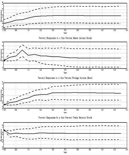
Matrix D is estimated with the diagonal normalized to one to find contemporaneous

innovations to 1% structural shocks. Estimated export revenue response functions are reported

in Figure 4.

*Figure 4*

A 1% depreciation shock decreases tourism export revenue contemporaneously followed

by an increase after one quarter and converging to equilibrium after six quarters. The short term

exchange rate elasticity is insignificant while the long term is marginally insignificant. Tourism

export revenue exhibits a robust positive response to foreign income and its own shocks.

Order of the import spending model y_t =[ΔE_t ΔM_t ΔY_t]' is justified in the same manner.

Both AIC and BIC choose k = 1 but to remove any remaining serial correlation k = 4 is utilized

as with export revenue.

) 0017 . 0 ( 0319 . 0 E t E

t = u

ε ) 0053 . 0 ( ) 0035 . 0 ( 0442 . 0 0032 . 0 M t E t M

t = u + u

ε ) 0008 . 0 ( ) 0005 . 0 ( ) 0006 . 0 ( 0068 . 0 0016 . 0 0002 .

0 tY

M t E

t Y

t = u + u + u

ε

The estimated import spending response functions are in Figure 5.

*Figure 5*

Responses are insignificant but import spending would appear to decrease

contemporaneously with a 1% depreciation shock, increasing after four quarters, and converging

to equilibrium after ten quarters. Import tourism spending also exhibits robust positive responses

to home income and its own shocks.

Consolidating results, the tourism balance of trade deteriorates initially following dollar

depreciation, improves after one quarter, and converges to the steady state after ten quarters.

Short term deterioration of the balance of trade is insignificant while the long term improvement

of the balance of trade is within the 90% confidence interval. There is no J-curve but there is a

lagged exchange rate effect on export revenue.

For comparison, in the balance of trade model y_t = [ΔE_tΔB_tΔY_tΔY_t*]' the order of

t

y is chosen assuming the exchange rate is not contemporaneously affected by shocks to the

balance of trade or home or foreign income, and the balance of trade is not contemporaneously

affected by shocks to home or foreign income. Home income is assumed not contemporaneously

affected by foreign income shocks. While higher foreign income may lead to export demand and

income growth in the long term, the effect after a few quarters would be negligible.

) 0008 . 0 ( 0147 . 0 E t E

t = u

ε ) 0026 . 0 ( ) 0041 . 0 ( 0418 . 0 0008 .

0 _tE _tB

B

t = u + u

ε ) 0020 . 0 ( ) 0032 . 0 ( ) 0036 . 0 ( 0383 . 0 0012 . 0 0169 .

0 _tE _tB _tY

Y

t = u + u + u

ε

(

)

(

) (

) (

)

0066 . 0 0000 . 0 0010 . 0 0002 . 0 * * Y t Y t B t E t Y

t =− u − u + u + u

ε

The choice of k = 4 is determined by the AIC. Matrix D with diagonal element normalized to

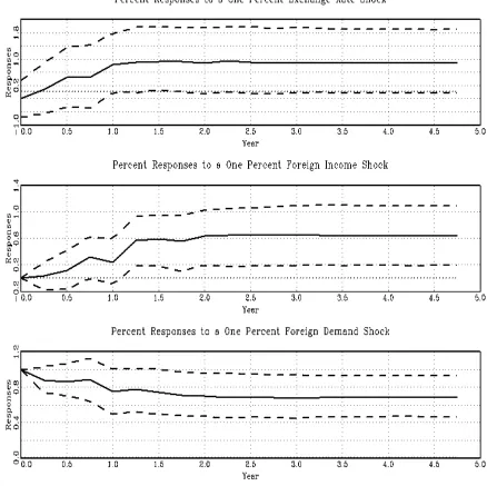
one is estimated and the balance of trade response functions are in Figure 6.

*Figure 6*

The balance of trade appears to increase contemporaneously with a 1% depreciation

shock but the response is insignificant. The response becomes significant after four quarters and

converges to long term equilibrium after eight quarters. There is no evidence of a J-curve but

depreciation raises the balance of trade. The balance of trade exhibits a robust positive response

to a positive home income shock that becomes insignificant after four quarters. The balance of

trade of tourism also exhibits a robust positive response to shocks to foreign income and itself.

The separate estimates provide more detailed response dynamics.

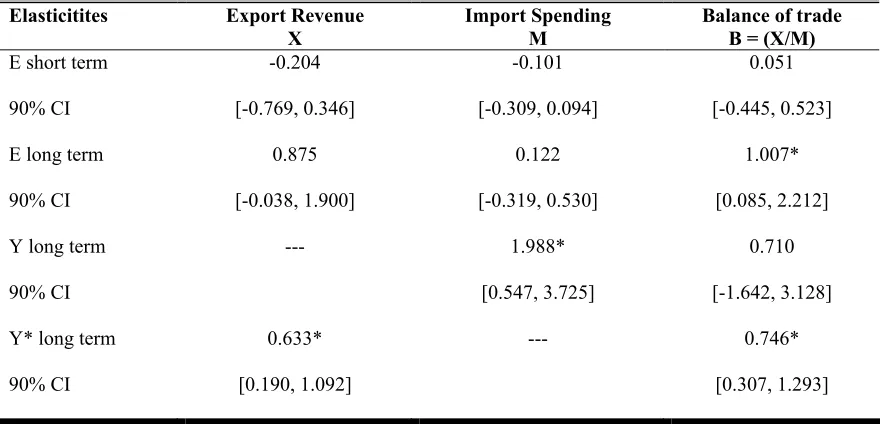
Long term exchange rate elasticities are a2 = 0.875 for tourism export revenue in (5) and

b2 = 0.122 for import tourism spending in (6). The derived exchange rate elasticities are ηx =

-0.875 and ηm = -0.878. The Marshall-Lerner condition is satisfied at the initial balance of trade

X/M = 0.591 where |ηx|(X/M) + |ηm| = 1.395 > 1 and at the 1.023 mean X/M where |ηx|(X/M) +

|ηm| = 1.774 > 1.

Short and long term exchange rate elasticities and long term income elasticities are

term tourism balance of trade. Foreign tourists coming to the US are more sensitive to the

exchange rate than US tourists going abroad while US tourists are much more sensitive to their

income. Aggregating the trade data disguises the strong income effect for US tourists.

*Table 2*

4. Conclusion

The present structural vector autoregressive model uncovers long term positive

depreciation effects of nominal dollar depreciation innovations on the US tourism balance of

trade. Foreign tourists into the US are more sensitive to the exchange rate than US tourists going

abroad while US tourists are more sensitive to income. There is no evidence of a J-curve in the

US tourism balance of trade.

The separate estimates of export revenue and import spending provide a more detailed

picture of the underlying dynamic adjustment to exchange rate shocks. Specifically, the balance

Table 1. Unit Root Pretests

Variable Specification ADFc ADFc,t

X Level -2.16 -1.15

Differenced -12.80*** -13.22***

M Level -1.98 -0.91

Differenced -14.36*** -14.65***

E Level -1.06 -1.86

Differenced -10.86*** -10.93***

Y Level -4.91*** -2.09

Differenced -4.88*** -9.28***

Y* Level -2.12 -1.69

Differenced -5.30*** -5.48***

Note: The number of lags is chosen by the Schwarz Information Criterion (BIC). ADFc and ADFc,t refer to ADF-t

statistics when an intercept is included and when an intercept and time trend are included. *, ** and *** indicate the null hypothesis of unit root is rejected at 10%, 5% and 1% level. Asymptotic critical values are from Harris (1992).

Table 2. Short and Long Term Exchange Rate and Income Elasticities

Elasticitites Export Revenue

X

Import Spending M

Balance of trade B = (X/M)

E short term

90% CI

-0.204

[-0.769, 0.346]

-0.101

[-0.309, 0.094]

0.051

[-0.445, 0.523]

E long term

90% CI

0.875

[-0.038, 1.900]

0.122

[-0.319, 0.530]

1.007*

[0.085, 2.212]

Y long term

90% CI

--- 1.988*

[0.547, 3.725]

0.710

[-1.642, 3.128]

Y* long term

90% CI

0.633*

[0.190, 1.092]

--- 0.746*

[0.307, 1.293]

Figure 1. Variable Series

0 1 2 3 4 5 6 7 8 9

1973Q1 1976Q1 1979Q1 1982Q1 1985Q1 1988Q1 1991Q1 1994Q1 1997Q1 2000Q1 2003Q1 2006Q1

lnX lnM lnE lnY lnY*

Figure 2. Differences of Variable

-0.3 -0.2 -0.1 0 0.1 0.2 0.3 0.4

1973Q2 1976Q2 1979Q2 1982Q2 1985Q2 1988Q2 1991Q2 1994Q2 1997Q2 2000Q2 2003Q2 2006Q2

Figure 3. Differences of Variable

-0.15 -0.1 -0.05 0 0.05 0.1 0.15 0.2

1973Q2 1976Q2 1979Q2 1982Q2 1985Q2 1988Q2 1991Q2 1994Q2 1997Q2 2000Q2 2003Q2 2006Q2

Figure 4. Impulse Response Function Estimates of Export Revenue

Figure 5. Impulse Response Function Estimates of Import Spending

Figure 6. Impulse Response Function Estimates of the Balance of trade

References

Ardalani, Z. and M. Bahmani-Oskoosee (2007) Is there a J-Curve at the Industry Level?

Economics Letters, 6, 1-12.

Bahmani-Oskooee, M. and T. J. Brooks (1999) Bilateral J-curve between US and Her Trading Partners, Weltwirtschaftliches Archiv, 135, 156-65.

Bahmani-Oskooee, M. and M. Malixi (1992) More evidence on the J-curve from LDCs, Journal

of Policy Modeling, 14, 641-53.

Bahmani-Oskooee, M. and A. Ratha (2004) The J-Curve: A Literature Review, Applied

Economics, 36, 1377-98.

Boyd, D., G. M. Caporale, and R. Smith (2001) Real Exchange Rate Effects on the Balance of Trade: Cointegration and the Marshall-Lerner Condition, International Journal of Finance and Economics, 6, 187-200.

Crouch G. L. (1994) The Study of International Tourism Demand: A Review of Findings,

Journal of Travel Research, 33, 12-23.

Demirden, T. and I. Pastine (1995) Flexible exchange rates and the J-curve: An alternative approach, Economics Letters, 48, 373-77.

Doroodian, K., C. Jung, and R. Boyd (1999) The J-curve effect and US agricultural and industrial trade, Applied Economics, 31, 687-95.

Dupont, B., A. Gandhi, and T. Weiss (2008) The American Invasion of Europe: The Long Term

Rise in Overseas Travel, 1820-2000, NBER Working Paper, 13977.

Goldstein, M. and M. S. Khan (1978) The Supply and Demand for Exports: a Simultaneous Approach, The Review of Economics and Statistics, 60, 275-86.

Goldstein, M. and M. S. Khan (1985) Income and Price Effects in Foreign Trade, in Handbook

of International Economics, Vol. 2 (Ed.) R. Jones and P. Kenen, Amsterdam: Elsevier.

Harris, R. I. D. (1992) Testing for Unit Roots using the Augmented Dickey-Fuller Test: Some Issues Relating to the Size, Power and the Lag Structure of the Test, Economics letters,

38, 381-86.

Harrop, J. (1973) On the Economics of Tourist Boom, Bulletin of Economic Research, May,

55-72.

Haynes, S. and J. Stone (1982) Impact of the Terms of Trade on the U.S. Trade Balance: A Reexamination, The Review of Economics and Statistics, 64, 702-06.

Hazari, B. R. (1995) Tourism and Growth in a Dynamic Model of Trade, The Journal of

Hazari, B. R. and A-Ng (1993) An Analysis of Tourists' Consumption of Non-traded Goods and

Services on the Welfare of the Domestic Consumers, International Review of Economics

& Finance, 2, 43-58.

Hazari B. R. and J. J. Nowak (2003) Tourism, Taxes and Immiserization: A Trade Theoretic Analysis, Pacific Economic Review, 8, 279-87.

Hazari, B. R. and P. M. Sgro (2004) Tourism, Trade and National Welfare, Elsevier.

Houthakker, H. S. and S. P. Magee (1969) Income and Price Elasticities in World Trade, The

Review of Economics and Statistics, 51, 111-25.

Junz, H. B. and R. R. Rhomberg (1973) Price-competitiveness in Export Trade among Industrial

Countries, The American Economic Review, 63, 412-18.

Magee, S. P. (1973) Currency Contracts, Pass Through and Depreciation, Brooking Papers on

Economic Activity, 1, 303-25.

Magee, S. P. (1975) Prices, Income and Foreign Trade: A Survey of Recent Economic Studies, in International trade and finance: Frontiers for research (Ed.) P. B. Kenen, Cambridge: Cambridge University Press.

Meade, E. E. (1988) Exchange Rates, Adjustment, and the J-curve, Federal Reserve Bulletin, October, 633-44.

Onafowora, O. (2003) Exchange Rate and Trade Balance in East Asia: Is there a J-curve?

Economics Bulletin, 5, 1-13.

Rhomberg, R. R. (1973) Towards a General Trade Model, in The International Linkage of

National Economic Models (Ed.) R. J. Ball, Amsterdam: North-Holland.

Rose, A. K. (1991) The role of Exchange Rates in a Popular Model of International Trade: Does

the ‘Marshall-Lerner’ Condition Hold? Journal of International Economics, 30, 301-16.

Rose, A. K. and J. L. Yellen (1989) Is there a J-curve? Journal of Monetary Economics, 24, 53-68.

Rosensweig, J. A. (1988) Elasticities of Substitution in Caribbean Tourism Demand, Journal of

Development Economics, 29, 89-100.

Rosensweig, J. A. and P. D. Koch (1988) The US Dollar and the ‘Delayed J-curve’, Economic

Review, July/August, Federal Reserve of Atlanta.

Senhadji, A. S. (1998a) Dynamics of the Trade Balance and the Terms of Trade in LDCs: the S-curve, Journal of International Economics, 46, 105-31.

Senhadji, A. S. (1998b) Time Series Estimation of Structural Import Demand Equations: A

Senhadji, A. and C. E. Montenegro (1999) Time Series Analysis of Export Demand Equations: A

Cross-Country Analysis, International Monetary Fund Staff Papers, 46, 259-73.

Sims, C. (1980) Macroeconomics and Reality, Econometrica, 48, 1-48.

Socher, K. (1986) Tourism in the Theory of International Trade and Payments, Tourism Review,

41, 24-26.

Song, H., S. F. Witt and G. Li (2009) The Advanced Econometrics of Tourism Demand, New

York: Routledge.

Vogt, M. G. (2008) Determinants of the Demand for US Exports and Imports of Tourism,

Applied Economics, 40, 667-72.

World Tourism Organization (2008) UNWTO World Tourism Barometer 6.

Appendix

Tourism export revenue X is the product of the quantity of export in tourism qx and the

price of domestic tourism p. Import spending on tourism M is the product of the quantity of

import in tourism qm and the price of international tourism in term of home currency Ep*.

Export revenue of the home country is

X = pqx (1)

Import spending of the home country is

M = Ep*qm (2)

Totally differentiate (1) and (2) to find

dX = pdqx + qxdp (3)

dM = Ep*dqm + p*qmdE + Eqmdp* (4)

Assume supply prices p and p* of international tourism do not change given perfectly elastic

supply curves over the range of quantity changes, dp = dp* = 0.

Elasticities of export and import demand are then

(

)

(

) (

)

d

q dqx x x =

η (5)

(

)

( ) ( )

η (6)

where (p/E) is the foreign price of US tourism and Ep* is the dollar price of international

tourism.

Equation (5) is expanded as

(

)

(

)

(

)

(

)

q dq_{x x}

x = ₋ 2

η =

(

)

(

)

q dq_{x x} x

− =

η (7)

Rearranging (7) x x x q E dE

dq ⎟η

⎠ ⎞ ⎜ ⎝ ⎛ −

Substitute (8) into (3) to rewrite dX in terms of export demand elasticity ηx,

x xpq E

dE

dX ⎟η

⎠ ⎞ ⎜ ⎝ ⎛ −

= = X

E dE x η ⎟ ⎠ ⎞ ⎜ ⎝ ⎛

− (9)

From (9) the elasticity of export tourism revenue a2 is related to the elasticity of export demand

as

(

)

(

)

E dE

X dX

a₂ = =−η (10)

Similarly from (6)

(

)

(

) ( )

η =

(

₍

₎

)

E dE

q dq_{m m}

(11) and rearranging m m m q E dE

dq ⎟η

⎠ ⎞ ⎜ ⎝ ⎛

= (12)

Substitute (12) into (4) to rewrite dM in terms of import demand elasticity ηm, to find

⎟ ⎠ ⎞ ⎜ ⎝ ⎛ + ⎟ ⎠ ⎞ ⎜ ⎝ ⎛ = E dE q Ep q Ep E dE

dM η_m * _m * _m = ⎟

(

)

⎠ ⎞ ⎜ ⎝ ⎛ m M E dE _η (13)

From (13), the elasticity of import tourism spending b2 is related to the elasticity of import

demand as

(

)

(

)

2 = = m + E

dE M dM