Modelling heterogeneity in response
behaviour towards a sequence of discrete
choice questions: a latent class approach
McNair, Ben J. and Hensher, David A. and Bennett, Jeff
The Australian National University
June 2010
Online at
https://mpra.ub.uni-muenchen.de/23427/
M
#16
2010
Environmental Management & Development
odelling heterogeneity in
response behaviour towards a
sequence of discrete choice
questions: a latent class
approach
Ben McNair, David A.
Hensher and Jeff Bennett
Crawford School of Economics and Government
THE AUSTRALIAN NATIONAL UNIVERSITY
http://www.crawford.anu.edu.au
Crawford School
of Economics and Government
Environmental Management and Development
Occasional Papers
are
published by the Environmental Management and Development Programme,
Crawford School of Economics and Government, Australian National University,
Canberra 0200 Australia.
These papers present peer-reviewed work in progress of research projects being
undertaken within the Environmental Management and Development Programme
by staff, students and visiting fellows.
The opinions expressed in these papers are those of the authors and do not
necessarily represent those of the Crawford School of Economics and
Government at The Australian National University.
ISSN 1447-6975
Acknowledgements
Modelling heterogeneity in response behaviour towards a sequence of
discrete choice questions: a latent class approach
Ben J. McNaira,*, David A. Hensherb and Jeff Bennetta
a Crawford School of Economics and Government, The Australian National
University, Canberra ACT 0200, Australia.
b
Institute of Transport and Logistics Studies, Faculty of Economics and Business,
The University of Sydney, NSW 2006, Australia. [email protected]
* Corresponding author. Email address: [email protected]
Abstract There is a growing body of evidence in the non-market valuation literature
suggesting that responses to a sequence of discrete choice questions tend to violate the
assumptions typically made by analysts regarding independence of responses and
stability of preferences. Heuristics such as value learning and strategic
misrepresentation have been offered as explanations for these results. While a few
studies have tested these heuristics as competing hypotheses, none have investigated
the possibility that each explains the response behaviour of a subgroup of the
population. In this paper, we make a contribution towards addressing this research gap
by presenting an equality-constrained latent class model designed to estimate the
proportion of respondents employing each of the proposed heuristics. We demonstrate
the model on binary and multinomial choice data sources and find three distinct types
response behaviour may be a better way forward than attempting to identify a single
heuristic to explain the behaviour of all respondents.
Keywords Choice experiment; latent class; ordering effects; strategic response;
willingness-to-pay
Introduction
Stated choice methods have become an increasingly popular approach to estimating
social values for non-market goods. In particular, choice experiments, which were
originally applied in the transport (Hensher and Truong 1985) and marketing
(Louviere and Hensher 1983) contexts, have been adapted to estimate values for a
range of environmental (Bennett and Blamey 2001) and monopoly service (Beenstock
et al. 1998, Carlsson and Martinsson 2008a) attributes. Choice experiments typically
involve presenting respondents with a sequence of choice tasks, where respondents
indicate their preference between two or more attribute-based alternatives in each
task. The presentation of multiple choice tasks per respondent is preferred, and in
some cases necessary, because it greatly increases the statistical efficiency of
estimation and allows estimation of the distribution of preferences for a given
attribute over a population. The standard assumptions when modelling responses to
these questions are that each question is answered independently and truthfully and
that underlying preferences are initially well-formed and stable over the course of the
sequence. Yet, several studies have found that responses violate these assumptions, in
some cases causing estimates of willingness-to-pay (WTP) implied by various order
positions in a sequence to differ (Bateman et al. 2008b, Cameron and Quiggin 1994,
Day et al. 2009, Day and Pinto 2010, DeShazo 2002, Hanemann et al. 1991, McNair
et al. 2010a).
Several heuristics have been put forward as explanations for such results. One group
of heuristics predict that respondents consider alternatives accepted in previous
questions when making their choices. These heuristics have generally been based on
the prediction of neo-classical economic theory, recently highlighted by Carson and
questions in order to maximise the likelihood of implementation of their most
preferred alternative observed over the sequence. Another group of heuristics revolve
around the idea that respondents have poorly-formed preferences that are influenced
by the information observed in choice tasks. This phenomenon was termed anchoring
(or starting-point bias) in the context of double-bounded contingent valuation surveys
in which the preferences stated in the first question differed from those stated in the
follow-up question (Boyle et al. 1985, Herriges and Shogren 1996). In longer
sequences of questions, the phenomenon has been characterised as value learning
(Plott 1996), which may be confined to the first question (Ariely et al. 2003), but
could extend further into a sequence of questions (for example in the form of a ‘good
deal / bad deal’ heuristic (Bateman et al. 2008b)).
A few studies have attempted to ascertain which of these heuristics best explains
responses in a given data set (Day et al. 2009, Day and Pinto 2010, DeShazo 2002,
McNair et al. 2010a), but none have investigated the possibility of heterogeneity in
response behaviour across respondents; that is, the possibility that each of the
proposed heuristics explains the response behaviour of a subgroup of respondents in
the survey (up to a probability). In this paper, we offer a contribution towards
addressing this research gap. The objective is to demonstrate, using both binary and
multinomial choice data, how an equality-constrained latent class (ECLC) model can
be used to account for discrete levels of heterogeneity in response behaviour towards
a sequence of choice questions. We use a framework similar to that previously used to
account for attribute non-attendance (Scarpa et al. 2009) and dual processing of
common-metric attributes (Hensher and Greene 2009). Classes of respondents are
defined by separate utility functions specified by restricting certain parameters to be
we ensure that class membership is determined by response behaviour towards a
sequence rather than by taste heterogeneity.
In the following section, we describe the heuristics that have been put forward in the
literature as potential explanations for ordering anomalies. We then detail the ECLC
model, the data source to which it is applied, and the results from the analysis before,
finally, drawing conclusions.
Background
Two of the standard assumptions when modelling responses to a sequence of stated
choice questions are that:
1. all respondents truthfully answer the question being asked; and
2. true preferences are stable over the course of a sequence of questions.
The focus of this paper is on accounting for response behaviour that violates one or
both of these assumptions in a way that affects estimates of willingness-to-pay
(WTP). Consequently, we do not seek to estimate the effects of any institutional
learning (Braga and Starmer 2005) or respondent fatigue.1 While these behavioural
processes have been shown to influence ‘noise’ in the data, manifest as changes in the
1 Two types of learning have been identified in the literature. The first, institutional learning, relates to
variance of the random error component (or, equivalently, scale)2 (Bradley and Daly
1994, Caussade et al. 2005, Holmes and Boyle 2005), there is no implied relationship
with WTP.
The various heuristics (or types of response behaviour) that do violate the standard
assumptions can be grouped into two broad categories – those that involve a violation
of the first standard assumption, and those that involve a violation of the second.
Strategic misrepresentation
Response behaviour that violates the first standard assumption can generally be
classified as strategic misrepresentation. It has long been recognised in neoclassical
economic theory that consumers may conceal their true preferences if it enables them
to obtain a public good at a lower cost (Samuelson 1954). More recently, Carson and
Groves (2007) highlighted the predictions of this theory in relation to stated choice
surveys. One of the predicted patterns of response behaviour is the rejection of an
alternative that is preferred to the status quo when a similar good was offered at a
lower cost in a previous choice task. This rejection increases the likelihood that the
respondent’s most preferred option across the sequence of choice tasks is
implemented. Bateman et al. (2008b) differentiate between strong strategic
misrepresentation, in which respondents always reject a good if it was offered at a
lower cost in a previous choice task, and weak strategic misrepresentation, in which
respondents weigh up the rejection against the perceived risk of the good not being
provided at the lower cost.
2 In the multinomial logit model, the scale parameter, λ, is an inverse function of the variance of the
DeShazo (2002) also argued that respondents do not answer questions independently,
but that they evaluate choice questions in terms of deviations from references points
based on previously accepted alternatives. DeShazo’s model shares the two main
predictions of the weak strategic misrepresentation hypothesis; first, that respondents
compare presented alternatives with alternatives accepted in previous choice tasks,
and, second, that respondents consider expected utility based on the probability of
provision. The prediction in both cases is that the WTP estimate implied by the first
question in a sequence will exceed the WTP estimates implied by subsequent
questions (assuming backward navigation through choice tasks is prevented).
Value learning
Response behaviour that violates the second standard assumption can generally be
classified as value learning (Plott 1996). Value learning heuristics revolve around the
idea that preferences are initially poorly-formed and are discovered in the process of
completing choice tasks. They generally predict that discovered preferences are
positively influenced by the cost levels presented in choice tasks. In
dichotomous-choice contingent valuation surveys, the outcome of such response behaviour has
been termed starting-point or anchoring bias (Boyle et al. 1985, Herriges and Shogren
1996). The focus in these short, one- or two-question sequences has been on the effect
on preferences of the cost level observed in the first choice task. With respect to the
longer sequences of questions typically employed in choice experiments, some
authors have maintained this focus on the effect of the first choice task (Ariely et al.
2003, Ladenburg and Olsen 2008), while others have put forward heuristics in which
the effect extends beyond the first task, potentially for the duration of the sequence of
questions. For example, Bateman et al. (2008b) describe a ‘good deal / bad deal’
chosen if its cost level is low (high) relative to the levels presented in previous choice
tasks.
If the value learning process is symmetric in terms of the effect of observed attribute
levels on preferences, then choice experiments can be designed in which this response
behaviour does not imply a relationship between question order and WTP.However,
this behaviour does imply a relationship between WTP and the cost levels (or bid
vector) used in the choice survey (Carlsson and Martinsson 2008b). As noted by
Bateman et al. (2008a), this relationship “fundamentally questions the underpinnings
of standard microeconomic theory, in effect suggesting that, at least to some degree,
prices determine values rather than vice versa.”
Empirical evidence
Turning to empirical evidence, a number of studies have found evidence of response
patterns associated with a single heuristic, whether it be a strategic misrepresentation
heuristic (Carson et al. 2009, Carson et al. 2006, Hensher and Collins 2010) or a value
learning heuristic (Ariely et al. 2003, Carlsson and Martinsson 2008b, Herriges and
Shogren 1996, Holmes and Boyle 2005, Ladenburg and Olsen 2008). However, only a
few have tested the heuristics discussed above as competing hypotheses to ascertain
which best explains responses in a given data set. DeShazo (2002) and Bateman et al.
(2008b) found evidence that supports a strategic misrepresentation heuristic in which
consideration is given to alternatives accepted in previous choice tasks and to the
perceived probability of provision. The weight of evidence found by Day and Pinto
(2010) supports a value learning heuristic, although the study found that no proposed
It appears that no studies have investigated the possibility of heterogeneity in response
behaviour across respondents; that is, the possibility that each of the proposed
heuristics explains the response behaviour of a subgroup of respondents in the survey.
In this paper, we offer a contribution towards addressing this research gap.
Method
While it may not be possible to identify whether a heuristic has been employed by
observing the responses of a single respondent, over a sufficiently large sample, it is
possible to identify the response patterns predicted by a given heuristic in terms of
relationships between responses and attribute levels observed by respondents in
previous choice tasks. We use an equality-constrained latent class (ECLC) model to
estimate the latent (or unknown) proportions of respondents behaving in accordance
with three heuristics based on the three types of response behaviour discussed above:
1. the standard assumptions (truthful, independent response with stable
preferences);
2. value learning; and
3. strategic misrepresentation.3
A random utility framework (McFadden 1974) is applied in which respondent utility
is equal to the sum-product of observed factors, x, and associated taste intensities, β,
plus unobserved factors, ε, which are i.i.d. according to the Extreme Value Type I
function. Following Hensher and Greene (2009), the resulting logit choice probability
function for the discrete choice from J alternatives can be written:
3 Even if respondents were directly asked to reveal their behaviour, the responses would be of little
Prob[choice j by individual i in choice task t | class q ] = Pit|q=
(
)
(
)
∑
= ′ ′ Jj itj jq
jq itj 1exp exp β β x x
The probability that individual i belongs to class q of Q is:
( )
( )
∑
= = Q q q q iq H 1exp exp θ θ, θQ=0
The log-likelihood function to be maximised is the sum over individuals of the log of
the expectation over classes of the joint probability of the sequence of T choices.
[
]
∑
∑
∏
∑
= = = = = = N i Tt itq
Q
q iq
N
i Pi H P
L 1ln 1ln 1 1 |
ln
In order to simplify the approach, the standard attributes, x, are defined so that they
take the value zero in the status quo utility function. To achieve this, we simply define
the attributes in terms of changes relative to the status quo. The reason for this
redefinition becomes clearer in the discussion to follow.
The Q classes are defined by separate parameter vectors, βjq. Parameters are
constrained to take the value zero in certain classes, but the non-zero parameters to be
estimated are constrained to take the same value across classes (i.e., they are assumed
to be generic). These Q vectors effectively translate to Q sets of utility functions to
which respondents are assigned up to a probability to maximise the log-likelihood
function.
In this study, Q=3 sets of utility functions are specified to capture the response
patterns associated with each of the three classes of response behaviour. Given that
the literature contains variants on each hypothesis, there is likely to be some argument
about how the utility functions should be specified for each class. While we do not
described below are the most suitable for this study based on the weight of evidence
in the literature and model fit testing. They are tailored to analyse responses to stated
choice surveys in which similar goods are offered at very different prices over the
course of a sequence. Such surveys arise in non-market valuation settings where
significant heterogeneity is expected in the distribution of WTP for a public project
over the population, but the set of credible project options are viewed as similar. The
consequence is that value learning and strategic behaviour tend to be driven mainly by
the cost attribute. Our utility functions are specified accordingly, however, the
approach could be expanded to incorporate the effects of other attributes.
Standard assumptions (Class 1)
The utility functions specified for the latent class of respondents behaving in
accordance with the standard assumptions are the conventional sum-product of the k
attributes as they appear in the choice task being answered and their associated taste
intensities.
Uit,SQ,class1 = β1x1,it,SQ + … + βkxk,it,SQ
Uit,ALT,class1 = β0 + β1x1,it,ALT + … + βkxk,it,ALT
Value learning (Class 2)
The second latent class represents those responding in accordance with a value
learning heuristic. We focus on the role of cost levels in value learning. Cost levels
are generally considered to be the main influence in the value learning process,
particularly in stated choice surveys in which similar goods are offered at very
different prices over the course of a sequence. We specify utility functions that
capture the response patterns of this group by allowing the alternative-specific
including the current choice task.4 This equal-weight average was found to result in
better model fit on our data source than a specification weighted towards more recent
observations. The length of the sequence in our data source was just four choice tasks.
In longer sequences, perfect recall is less likely and a weighted specification may be
preferred (for example Day et al. 2009). The cost level in the current choice task is
included in the average to accommodate the prediction of coherent arbitrariness
(Ariely et al. 2003), anchoring and starting-point bias (Herriges and Shogren 1996)
that the cost level observed in the first choice task will influence preferences prior to
response. The utility functions are as follows.
Uit,SQ,class2 = β1x1,it,SQ + … + βkxk,it,SQ
Uit,ALT,class2 = β0 + β1x1,it,ALT + … + βkxk,it,ALT + βk+1zit,ALT
where
zitj = zoitj – žj
zoitj = the average of cost levels observed up to and including the current
choice task
žj = the average of cost levels in the sample (across all respondents and
all choice tasks)
The purpose of žjis econometric rather than behavioural. It simply ‘normalises’ the
average observed cost variable by ensuring its sample mean is approximately zero.
4 The main variation within the group of value learning heuristics lies in the length of the sequence of
This prevents the latent class model from using the coefficient, βk+1, to infer
heterogeneity in taste across classes, thus ensuring the model estimates only
heterogeneity in response behaviour towards the sequence of questions.
Strategic misrepresentation (Class 3)
In a third class of response behaviour, we specify utility functions that capture the
response patterns predicted by a strategic misrepresentation heuristic. The heuristic
has two features. The first is that respondents compare alternatives to those accepted
in previous choice tasks. In particular, they choose the status quo option not only
when the status quo is preferred to the alternatives, but, potentially, also when a
previously accepted alternative is preferred to the alternatives currently on offer. We
assume that respondents effectively replace the status quo with a reference alternative
once they have expressed a preference for an alternative over the status quo. We
define the reference alternative as the highest-cost alternative previously accepted in
the sequence. Over the range of cost and WTP levels that matter, this reference
alternative yields the highest expected utility (based on the provision probabilities
discussed below) of all previously accepted alternatives.5
The second feature of this heuristic is that respondents consider the probability of
provision. When a similar good is offered at very different cost levels over the course
of a sequence of choice tasks, respondents may assume that higher-cost goods are
more likely to be provided because the agency is more likely to proceed with the
5 We showed by simulation that, if the good being offered is sufficiently similar across tasks, the
project the higher is respondents’ stated WTP. We assume the perceived probability
of project provision is equal to the ratio of the maximum cost level accepted and the
maximum cost level observed.6 Consider the case where a project option priced at
$4,000 is accepted in the first of a sequence of binary choice tasks. If a project option
priced at $8,000 is presented in the second task, then the perceived probability of
project provision is revised to 50 per cent. The respondent is faced with a trade-off.
The perceived probability of provision can be increased to 100 per cent, but at the cost
of accepting the more expensive ($8,000) alternative. If the alternative is accepted, it
becomes the reference alternative in the next choice task. Alternatively, if a project
option priced at $2,000 is presented in the second choice task, then the choice does
not influence the probability of project provision (and the respondent will accept the
$2,000 alternative assuming the goods are sufficiently similar).
The utility equations represent the expected utilities from the reference and current
alternatives.7
Uit,SQ,class3 = pit,SQ(β0 + β1xa1,it + … + βkxak,it)
Uit,ALT,class3 = pit,ALT(β0 + β1x1,it,ALT + … + βkxk,it,ALT)
where
xait= the levels of attributes in the highest-cost alternative accepted in previous
choice tasks (xa1,it is the maximum cost level accepted in previous choice
tasks)
6 The perceived probability of provision is unlikely to ever be 100 per cent due to uncertainty about
others’ preferences and the advisory nature of most surveys. However, it is the relative probabilities, rather than the absolute probabilities, that are important in determining the choice probabilities.
pit,SQ = xa1,it/xo1,it
xo1,it = the maximum cost level observed up to and including the current choice
task
pit,ALT = max[pit,SQ , x1,it,ALT/xo1,it]
The importance of defining the standard attributes in terms of changes relative to the
status quo now becomes clear. If a respondent has chosen the status quo in all choice
tasks to a given point, then xa1,it=0, pit,SQ=0 and Uit,SQ,class3= Uit,SQ,class1= Uit,SQ,class2=0.
In the first question in a sequence, the class 3 utility functions are identical to those in
Class 1 since pit,SQ=0 and pit,ALT=1. Once a respondent has chosen an alternative over
the status quo, that alternative replaces the status quo as the reference point and
Uit,SQ,class3>0. Alternatives presented in subsequent choice tasks are accepted if the
expected utility from choosing the alternative exceeds the expected utility from
choosing the reference alternative.
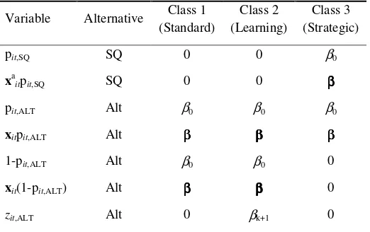
Class structure in the equality-constrained latent class model
The three sets of utility functions are operationalised in the latent class model by three
separate sets of restrictions on a ‘master’ utility function. Certain parameters are
restricted to be zero and certain parameters are restricted to be equal both within and
across classes as shown in Table 1. The alternative-specific constants and the standard
attributes, x, are divided into two parts – one multiplied by pit,ALT and another by 1-
pit,ALT. In Classes 1 and 2, coefficients on attributes multiplied by pit,ALT and 1- pit,ALT
are assumed to be equal so that they represent the marginal utility of the standard
attribute without consideration of the probability of provision. In Class 3, the
coefficients on attributes multiplied by 1- pit,ALT are set to zero so that utility depends
to hold zero value in Classes 1 and 2 (in which previously accepted alternatives are
ignored), but in Class 3, they are assumed to have the same taste intensities as the
equivalent variables in the non-status-quo alternatives in the current choice task. All
[image:19.612.107.368.204.368.2]non-zero attributes are assumed to take the same value across classes.
Table 1: Class structurea
Variable Alternative Class 1 (Standard)
Class 2 (Learning)
Class 3 (Strategic) pit,SQ SQ 0 0 β0
xaitpit,SQ SQ 0 0 ββββ
pit,ALT Alt β0 β0 β0
xitpit,ALT Alt β βββ ββββ ββββ
1-pit,ALT Alt β0 β0 0
xit(1-pit,ALT) Alt ββ ββ ββββ 0
zit,ALT Alt 0 βk+1 0
aββββ refers to a coefficient vector, β1, β2,…, βk, associated with x1,…, xk.
Data
We implement the model on data from a survey of homeowners in the Australian
Capital Territory (ACT) in 2009. The main objective of the survey was to establish
homeowners’ willingness to pay to have overhead electricity and telecommunications
wires in their suburb replaced by new underground wires. We provide a brief
overview herein and refer readers to McNair et al. (2010b) for details.
Data from two elicitation formats used in the survey are analysed in this study. The
first format comprised a sequence of four binary choice tasks in which respondents
were presented with a description of their current (overhead) service and one
undergrounding alternative (the binary choice format). The second format also
comprised a sequence of four choice tasks, but each task contained the current service
used to describe the alternatives and the levels assigned to those attributes are
presented in Table 2. The value of the alternative label embodies all of the benefits of
undergrounding other than supply reliability benefits, including the amenity and
safety benefits that qualitative questions showed to be the major household benefits
from undergrounding. The restricted range of credible levels for supply reliability
attributes meant that similar goods were offered at very different prices over the
course of the choice task sequences. Consequently, opportunities for strategic
misrepresentation may have been relatively obvious and, potentially, value learning
[image:20.612.108.492.325.616.2]may have been exacerbated.
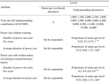
Table 2: Attributes and levels
Levels Attribute Status quo (overhead)
alternative Undergrounding alternatives
Your one-off undergrounding
contribution (AUD 2009) 0
1,000, 1,100, 2,000, 2,100, 2,800, 3,000, 3,900, 4,000, 6,000, 6,200,
8,000, 8,200, 11,800, 12,000, 15,900, 16,000 Power cuts without warning:
Number of power cuts each
five years Set by respondent
Proportions of status quo level: 0.25, 0.5, 0.75, 1 a,b Average duration of power cuts Set by respondent Proportions of status quo level:
0.33, 0.66, 1.33, 1.66 a
Power cuts with written notice (occurring in normal business hours):
Number of power cuts each
five years Set by respondent
Proportions of status quo level: 0.2, 0.4, 0.6, 0.8 a,b Average duration of power cuts Set by respondent Proportions of status quo level:
0.33, 0.66, 1.33, 1.66 a
a Rounded to the nearest integer; b Absolute levels (0, 1 and 2) were assigned where respondents chose
very low status quo levels (1 or less).
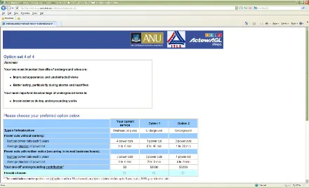
Two blocks of four choice tasks were constructed in the multinomial choice format to
minimise the correlation between attribute levels and block assignment.8 The binary
design was created by splitting these two blocks into four blocks of four binary choice
tasks. An example of a choice task from the multinomial choice format is presented in
[image:21.612.110.550.204.472.2]Figure 1.
Figure 1: Example of a choice task
Some 292 respondents completed the web-based questionnaire in the binarychoice
format and 290 in the multinomial choice format. Importantly, the questionnaire did
not allow respondents to navigate back through the sequence of choice tasks. It was
programmed to cycle through the various sample splits, blocks and choice task
orderings to ensure approximately equal representation across choice observations.
8 Bayesian priors were derived from pilot responses and from NERA and ACNielsen (2003). Default
As many as 30 per cent of respondents completing the binary format and 24 per cent
of respondents completing the multinomial format chose the status quo scenario in all
four choice tasks. The response behaviour of this group is difficult to determine
because, if the value placed on undergrounding by a respondent is sufficiently low,
then all three heuristics result in the same pattern of responses - selection of the status
quo in every task. These respondents are omitted from the analysis in this paper to
ensure that the method can be demonstrated effectively. We expect the method could
be applied to full survey data sets in other studies where such responses represent a
lower proportion of the sample.
An important part of the method is the manipulation of variables prior to estimation.
We used a spreadsheet to create the normalised average observed cost variable, zit,ALT,
the provision probability proxies for the reference and current alternatives, pit,SQ and
pit,ALT, the attribute levels associated with the highest-cost alternative previously
accepted, xait, and the maximum cost level observed up to and including the current
choice task, xo1,it.
Results
A summary of the ECLC model results for the binary (Model 1) and multinomial
(Model 2) formats is presented in Table 3 with full estimation results detailed in the
Appendix. The seven parameter estimates in each model have the expected sign where
they are significant at the 0.05 level. The positive coefficient on the normalised
average observed cost variable indicates that, within Class 2, the value placed on
undergrounding is influenced by the cost levels observed in previous choice tasks and
the current choice task. A respondent in this class is more likely to accept an
offered in the first choice task was priced at $6,000 than if it was priced at $2,000 (all
[image:23.612.111.539.149.420.2]else held constant).
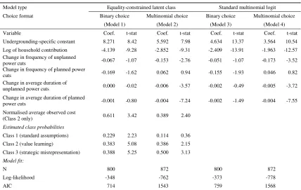
Table 3: Summary of estimation results
Model type Equality-constrained latent class Standard multinomial logit Choice format Binary choice Multinomial choice Binary choice Multinomial choice
(Model 1) (Model 2) (Model 3) (Model 4)
Variable Coef. t-stat Coef. t-stat Coef. t-stat Coef. t-stat Undergrounding-specific constant 8.271 8.42 5.592 7.98 4.634 13.37 3.564 10.54 Log of household contribution -4.139 -9.28 -2.852 -9.31 -2.409 -13.91 -1.963 -12.57 Change in frequency of unplanned
power cuts -0.067 -1.07 -0.153 -2.76 -0.051 -1.07 -0.173 -3.52 Change in frequency of planned power
cuts -0.169 -1.62 0.062 0.94 -0.155 -1.93 0.046 0.82 Change in average duration of
unplanned power cuts 0.000 -0.02 -0.006 -3.57 -0.002 -0.49 -0.005 -3.72
Change in average duration of planned
power cuts -0.001 -0.80 -0.004 -7.24 -0.002 -1.49 -0.004 -7.55 Normalised average observed cost
(Class 2 only) 0.611 3.42 0.389 2.40
Estimated class probabilities
Class 1 (standard assumptions) 0.229 2.23 0.114 0.36 Class 2 (value learning) 0.383 5.08 0.386 2.15 Class 3 (strategic misrepresentation) 0.388 5.25 0.500 3.13
Model fit:
N 800 872 800 872
Log-likelihood -348 -762 -373 -778
AIC 714 1543 759 1568
Turning to the estimated class probabilities, all except one are significant at the 0.05
level across the two models. Both models estimate that 39 per cent of respondents
behaved according to the value learning utility specification. The proportion behaving
in line with the strategic misrepresentation specification is estimated at 38 per cent in
the binary format and 50 per cent in the multinomial format. The class with the lowest
membership probability in both models was that based on the standard assumptions of
truthful response and stable preferences, with 23 and 11 per cent predicted by Model 1
and Model 2, respectively. No single class dominates either model, indicating
significant heterogeneity in the response behaviour towards both the binary and
format and response behaviour, with the class probabilities statistically
indistinguishable at the 0.05 level across the two models.
The log-likelihood values associated with the ECLC models indicate an improvement
in model fit over the standard multinomial logit (MNL) models (also presented in
Table 3). This improvement is expected given the additional parameters
accommodating heterogeneity in the ECLC models. Of greater interest is the
improvement in the AIC value, which accounts for parameter proliferation. The
improvement in this criterion suggests that accounting for heterogeneity in response
behaviour using the ECLC model is important even when model parsimony is
considered desirable.
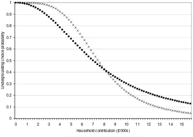
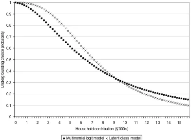
Turning to implications for welfare estimates, the undergrounding choice probability
(or bid acceptance) functions for the binary and multinomial choice format models are
shown in Figure 2 and Figure 3 (with all non-cost attributes are set at their sample
means). Estimates of mean total WTP, calculated as the areas under the
undergrounding choice probability curves, are not significantly different at the 0.05
level across the ECLC and MNL models. However, this may not be the case in other
data sources. The changes in the curves when moving from the MNL to the latent
class model are the net effect of two separate influences – the effect of accounting for
value learning (Class 2); and the effect of accounting for strategic misrepresentation
(Class 3). The overall effect on WTP depends on the magnitude of each of these
Figure 2: Undergrounding choice probability implied by models on binary choice format 0 0.1 0.2 0.3 0.4 0.5 0.6 0.7 0.8 0.9 1
0 1 2 3 4 5 6 7 8 9 10 11 12 13 14 15
Household contribution ($'000s)
U n d e rg ro u n d in g c h o ic e p ro b a b ili ty
Multinomial logit model Latent class model
The expected effect of accounting for value learning behaviour is an increase in
probabilities at lower costs and a decrease in probabilities at higher costs. The reason
is as follows. Average observed cost, z, is positively related to cost, x1, for a given set
of cost levels in previous choice tasks. Utility from undergrounding alternatives net of
the effect of average observed cost therefore needs to be higher at lower cost levels
and vice versa in order to adequately explain respondents’ choices. The latent class
model achieves this by altering the remaining parameters, β. The effect is a narrowing
Figure 3: Undergrounding choice probability implied by models on multinomial choice format 0 0.1 0.2 0.3 0.4 0.5 0.6 0.7 0.8 0.9 1
0 1 2 3 4 5 6 7 8 9 10 11 12 13 14 15
Household contribution ($'000s)
U n d e rg ro u n d in g c h o ic e p ro b a b ili ty
Multinomial logit model Latent class model
The expected effect of accounting for strategic misrepresentation is an increase in
undergrounding choice probability at all cost levels (albeit not in a linear fashion). For
a given set of parameters, β, the undergrounding choice probability for Class 3 is
always less than or equal to that for Class 1 since Uit,SQ,class3≥Uit,SQ,class1 and
Uit,ALT,class3≤ Uit,ALT,class1.9 Therefore, when switching from a Class 1 to a Class 3
utility specification, the parameters must be altered in such a way that increases the
undergrounding choice probability.
Conclusions
This paper presents an equality-constrained latent class (ECLC) model that can be
used to identify heterogeneity in response behaviour towards a sequence of choice
tasks. The illustrative evidence herein shows the model can be applied to choice data
from both binary and multinomial choice formats where a status quo alternative is
present and similar goods are offered at very different prices over the course of a
sequence of questions.
The ECLC models achieved an improvement in fit over standard multinomial logit
(MNL) models, even based on information criteria that account for model parsimony.
Estimates of total willingness-to-pay were statistically indistinguishable between the
two types of model. However, this may not be the case in other data sources as it
depends on several factors including the relative mix of class probabilities.
Three distinct groups were identified in both the binary and multinomial choice data.
The group behaving in accordance with the standard assumptions was the smallest of
the three in both models, providing further evidence that the standard assumptions do
not adequately reflect the response behaviour of the majority of respondents in a
survey of this type. The heterogeneity in response behaviour identified herein may
explain the variation in findings across studies and the ambiguity of evidence within
studies (Day and Pinto 2010) that have attempted to identify a single heuristic that
best describes respondent behaviour towards a sequence of choice questions. It
suggests that the literature may never converge to agreement on a single heuristic. The
best way forward would appear to be to account for heterogeneity in response
behaviour. The method presented in this paper is one approach that could be used in
future studies. Clearly, other approaches are possible and this is likely to be a fertile
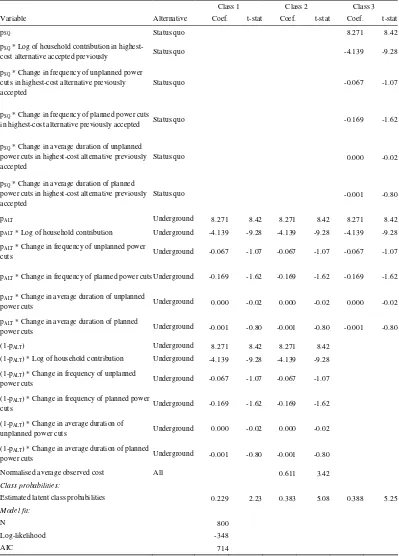
Appendix
Table 4: Equality-constrained latent class model on binary choice data (Model 1)
Class 1 Class 2 Class 3 Variable Alternative Coef. t-stat Coef. t-stat Coef. t-stat
pSQ Status quo 8.271 8.42
pSQ * Log of household contribution in
highest-cost alternative accepted previously Status quo -4.139 -9.28
pSQ * Change in frequency of unplanned power
cuts in highest-cost alternative previously accepted
Status quo -0.067 -1.07
pSQ * Change in frequency of planned power cuts
in highest-cost alternative previously accepted Status quo -0.169 -1.62
pSQ * Change in average duration of unplanned
power cuts in highest-cost alternative previously accepted
Status quo 0.000 -0.02
pSQ * Change in average duration of planned
power cuts in highest-cost alternative previously accepted
Status quo -0.001 -0.80
pALT Underground 8.271 8.42 8.271 8.42 8.271 8.42
pALT * Log of household contribution Underground -4.139 -9.28 -4.139 -9.28 -4.139 -9.28
pALT * Change in frequency of unplanned power
cuts Underground -0.067 -1.07 -0.067 -1.07 -0.067 -1.07
pALT * Change in frequency of planned power cuts Underground -0.169 -1.62 -0.169 -1.62 -0.169 -1.62
pALT * Change in average duration of unplanned
power cuts Underground 0.000 -0.02 0.000 -0.02 0.000 -0.02
pALT * Change in average duration of planned
power cuts Underground -0.001 -0.80 -0.001 -0.80 -0.001 -0.80
(1-pALT) Underground 8.271 8.42 8.271 8.42
(1-pALT) * Log of household contribution Underground -4.139 -9.28 -4.139 -9.28
(1-pALT) * Change in frequency of unplanned
power cuts Underground -0.067 -1.07 -0.067 -1.07
(1-pALT) * Change in frequency of planned power
cuts Underground -0.169 -1.62 -0.169 -1.62
(1-pALT) * Change in average duration of
unplanned power cuts Underground 0.000 -0.02 0.000 -0.02
(1-pALT) * Change in average duration of planned
power cuts Underground -0.001 -0.80 -0.001 -0.80
Normalised average observed cost All 0.611 3.42
Class probabilities:
Estimated latent class probabilities 0.229 2.23 0.383 5.08 0.388 5.25
Model fit:
N 800
Log-likelihood -348
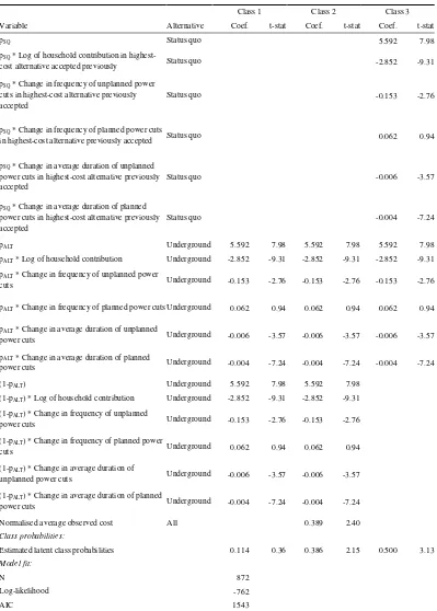
Table 5: Equality-constrained latent class model on multinomial choice data (Model 2)
Class 1 Class 2 Class 3
Variable Alternative Coef. t-stat Coef. t-stat Coef. t-stat
pSQ Status quo 5.592 7.98
pSQ * Log of household contribution in
highest-cost alternative accepted previously Status quo -2.852 -9.31
pSQ * Change in frequency of unplanned power
cuts in highest-cost alternative previously accepted
Status quo -0.153 -2.76
pSQ * Change in frequency of planned power cuts
in highest-cost alternative previously accepted Status quo 0.062 0.94
pSQ * Change in average duration of unplanned
power cuts in highest-cost alternative previously accepted
Status quo -0.006 -3.57
pSQ * Change in average duration of planned
power cuts in highest-cost alternative previously accepted
Status quo -0.004 -7.24
pALT Underground 5.592 7.98 5.592 7.98 5.592 7.98
pALT * Log of household contribution Underground -2.852 -9.31 -2.852 -9.31 -2.852 -9.31
pALT * Change in frequency of unplanned power
cuts Underground -0.153 -2.76 -0.153 -2.76 -0.153 -2.76
pALT * Change in frequency of planned power cuts Underground 0.062 0.94 0.062 0.94 0.062 0.94
pALT * Change in average duration of unplanned
power cuts Underground -0.006 -3.57 -0.006 -3.57 -0.006 -3.57
pALT * Change in average duration of planned
power cuts Underground -0.004 -7.24 -0.004 -7.24 -0.004 -7.24
(1-pALT) Underground 5.592 7.98 5.592 7.98
(1-pALT) * Log of household contribution Underground -2.852 -9.31 -2.852 -9.31
(1-pALT) * Change in frequency of unplanned
power cuts Underground -0.153 -2.76 -0.153 -2.76
(1-pALT) * Change in frequency of planned power
cuts Underground 0.062 0.94 0.062 0.94
(1-pALT) * Change in average duration of
unplanned power cuts Underground -0.006 -3.57 -0.006 -3.57
(1-pALT) * Change in average duration of planned
power cuts Underground -0.004 -7.24 -0.004 -7.24
Normalised average observed cost All 0.389 2.40
Class probabilities:
Estimated latent class probabilities 0.114 0.36 0.386 2.15 0.500 3.13
Model fit:
N 872
Log-likelihood -762
References
Ariely D, Loewenstein D and Prelec D (2003) 'Coherent arbitrariness': stable demand curves without stable preferences. Quarterly Journal of Economics 118(1): 73-105
Bateman I J, Burgess D, Hutchinson W G and Matthews D I (2008a) Learning design contingent valuation (LDCV): NOAA guidelines, preference learning and coherent arbitrariness. Journal of Environmental Economics and Management 55: 127-141
Bateman I J, Carson R T, Day B, Dupont D, Louviere J J, Morimoto S, Scarpa R et al (2008b) Choice set awareness and ordering effects in discrete choice experiments. CSERGE Working Paper EDM 08-01
Beenstock M, Goldin E and Haitovsky Y (1998) Response bias in conjoint analysis of power outages. Energy Economics 20: 135-156
Bennett J and Blamey R (2001) The Choice Modeling Approach to Environmental Valuation. Edward Elgar, Cheltenham, UK
Boyle K J, Bishop R C and Welsh M P (1985) Starting Point Bias in Contingent Valuation Bidding Games. Land Economics 61: 188-194
Bradley M and Daly A (1994) Use of the logit scaling approach to test for rank-order and fatigue effects in stated preference data. Transportation 21(2): 167-184
Braga J and Starmer C (2005) Preference anomolies, preference elicitation and the discovered preference hypothesis. Environmental and Resource Economics 32: 55-89
Cameron T A and Quiggin J (1994) Estimation using contingent valuation data from a "dichotomous choice with follow-up" questionnaire. Journal of Environmental Economics and Management 27: 218-234
Carlsson F and Martinsson P (2008a) Does it matter when a power outage occurs? A choice experiment study on the WTP to avoid power outages. Energy Economics 30(3): 1232-1245
Carson K S, Chilton S M and Hutchinson W G (2009) Necessary conditions for demand revelation in double referenda. Journal of Environmental Economics and Management 57(2): 219-225 Carson R T and Groves T (2007) Incentive and informational properties of preference questions.
Environmental and Resource Economics 37: 181-210
Carson R T, Groves T and List J (2006) Probabilistic influence and supplemental benefits: a field test of the two key assumptions behind using stated preferences. unpublished manuscript, Caussade S, Ortuzar J d D, Rizzi L I and Hensher D A (2005) Assessing the influence of design
dimensions on stated choice experiment estimates. Transportation Research Part B 39: 621-640
Day B, Bateman I J, Carson R T, Dupont D, Louviere J J, Morimoto S, Scarpa R et al (2009) Task Independence in Stated Preference Studies: A Test of Order Effect Explanations. CSERGE Working Paper EDM 09-14,
Day B and Pinto J L (2010) Ordering anomalies in choice experiments. Journal of Environmental Economics and Management doi:10.1016/j.jeem.2010.03.001
DeShazo J R (2002) Designing transactions without framing effects in iterative question formats. Journal of Environmental Economics and Management 43: 360-385
Hanemann W M, Loomis J and Kanninen B (1991) Statistical efficiency of double bounded dichotomous choice contingent valuation. American Journal of Agricultural Economics 73: 1255-1263
Hensher D A and Collins A T (2010) Interrogation of Responses to Stated Choice Experiments: Is there sense in what respondents tell us? Submitted to Journal of Choice Modelling
Hensher D A and Greene W H (2009) Non-attendance and dual processing of common-metric attributes in choice analysis: a latent class specification Empirical Economics (in press) Hensher D A and Truong T P (1985) Valuation of Travel Time Savings: A Direct Experimental
Approach. Journal of Transport Economics and Policy 19(3): 237-261
Herriges J A and Shogren J F (1996) Starting point bias in dichotomous choice valuation with follow-up questioning. Journal of Environmental Economics and Management 30: 112-131 Holmes T and Boyle K J (2005) Dynamic learning and context-dependence in sequential,
Ladenburg J and Olsen S B (2008) Gender-specific starting point bias in choice experiments: Evidence from an empirical study. Journal of Environmental Economics and Management 56: 275-285 Louviere J J and Hensher D A (1983) Using Discrete Choice Models with Experimental Design Data to
Forecast Consumer Demand for a Unique Cultural Event. Journal of Consumer Research 10(December): 348-361
McFadden D (1974) Conditional Logit Analysis of Qualitative Choice Behaviour. In: Zarembka P (ed) Frontiers in Econometrics, Academic Press, New York
McNair B J, Bennett J and Hensher D A (2010a) A comparison of responses to single and repeated discrete choice questions. Occasional Paper #14, Crawford School of Economics and Government, The Australian National University,
____ (2010b) Households' willingness to pay for undergrounding electricity and telecommunications wires. Occasional Paper #15, Crawford School of Economics and Government, The Australian National University,
NERA Economic Consulting and ACNielsen (2003) Willingness to pay research study. A report for ACTEW Corporation and ActewAGL, September
Plott C R (1996) Rational individual behavior in markets and social choice processes: the discovered preference hypothesis. In: Arrow K, Colombatto E, Perleman M and Schmidt C (ed) Rational foundations of economic behavior, Macmillan, London
Samuelson P A (1954) The pure theory of public expenditure. Review of Economics and Statistics 36: 387-389
Scarpa R, Gilbride T J, Campbell D and Hensher D A (2009) Modelling attribute non-attendance in choice experiments for rural landscape valuation. European Review of Agricultural Economics 36(2): 151-174
List of previous EMD Occasional Papers List of previous EMD Occasional Papers List of previous EMD Occasional Papers List of previous EMD Occasional Papers
!""!
# $ !% &
' ' & & !""(
) *
& !""(
+ &
, & -. / .'. 0
!""(
& & 0
1
2 !""3
& 2 & & ) 4 2
-' & /
0 !""3
+ &
5 6
- !""3
) # 7 8 &
+
-!""9
5 + & : 2
2 + ; 0 & 0&
1 # = 0 & 0 8
5 !""<
& 2 + 1 5 1
2 + 1= / =
- !""<
0 # 6 2 ' /
- # #
!""<
' &
-& !"">
?
. - . '
& !"%"
' 7 = & & =
. - . '