Munich Personal RePEc Archive
A (micro) course in microeconomic
theory for MSc students
Gaudeul, Alexia
22 May 2009
A (Micro) Course in Microeconomic Theory for
MSc Students
Alexia Gaudeul
∗May 23, 2009
Abstract
Those lecture notes cover the basics of a course in microeconomic theory for MSc students in Economics. They were developed over five years of teaching MSc Economic Theory I in the School of Economics at the University of East Anglia in Norwich, UK. The lectures differ from the standard fare in their emphasis on utility theory and its alternatives. A wide variety of exercises for every sections of the course are provided, along with detailed answers. Credit is due to my students for ‘debugging’ this material over the years. Specific credit for some of the material is given where appropriate.
JEL codes: A1, A23, D0.
Keywords: Economics, Microeconomics; Utility Theory; Game The-ory; Incentive TheThe-ory; Online Textbook; Lecture Notes, Study Guide, MSc.
∗Please direct comments and report mistakes to me at [email protected]. My website
is at http://agaudeul.free.fr.
1 PROGRAMME 2
1
Programme
The programme of this course is divided in three parts; choice under uncertainty, game theory and incentive theory. The whole of the course can be covered in sixteen hours of teaching, along with eight hours of workshops, over eight weeks. This is an intensive program that is designed both to cover the basics in each area and progress quickly to more advanced topics. The course is thus accessible to students with little background in economics, but should also challenge more advanced students who can focus on the later sections in each parts and concen-trate on the suggested readings. Exercises covering each part increase gradually in difficulty and are often of theoretical interest on their own. Detailed answers are provided.
This course may be complemented with lectures on consumer and firm theory, and on general equilibrium concepts. Those are not covered in those notes.
The main concepts that are covered in each part are listed below:
Choice under uncertainty (2×2 hours lectures, 1×2 hours workshop):
Rationality and axiomatic theories of choice. Expected utility theory: its foundations and applications. Experimental tests of expected utility theory. Alternatives to EUT: prospect theory, rank dependent expected utility theory, cumulative prospect theory, regret theory.
A large part of this topic is not covered in standard text books and this topic thus requires independent reading.
Game Theory (4×2 hours lectures, 2×2 hours workshops): Normal (or strategic)-Form Games. Dominance, Nash equilibrium, and mixed-strategy extensions. Extensive-Form Games. Information sets, subgame-perfect equilibria, and backward induction. Incomplete-information games, Bayesian Games, Bayesian-Nash equilibria, forward induction. Purifica-tion of mixed strategy equilibria. AucPurifica-tions. Repeated games and the Folk theorem.
Incentive Theory (2×2 hours lecture, 1×2 hours workshop): Principal-agent models. Adverse selection (hidden information). Moral hazard (hidden action). Second best and efficiency. Liability constraints. Risk aversion. Commitment. Repeated adverse selection. Hold up problem. Informed principal. Revelation principle. Direct Revelation Mechanism.
2
Textbooks:
The main texts for the course are:
• Kreps D.M., 1990, A course in Microeconomic Theory, FT/Prentice Hall (hereafter ‘Kreps’).
2 TEXTBOOKS: 3
• Mas-Colell A., M.D. Whinston and J.R. Green, 1995, Microeconomic The-ory, Oxford University Press (hereafter ‘Mas-Colell’).
CONTENTS 4
Contents
1 Programme 2
2 Textbooks: 2
I
Choice under uncertainty
9
3 Introduction 10
4 Readings 10
4.1 Textbook Readings . . . 10
4.2 Other general readings . . . 10
4.3 Articles . . . 11
5 Basic tools and notations 11 5.1 The objects of preference and choice . . . 11
5.2 Lotteries . . . 12
5.3 The Marschak-Machina Triangle . . . 14
6 Expected Utility Theory 15 6.1 The axioms of von Neumann and Morgenstern’s Expected Utility Theory . . . 15
6.1.1 Completeness . . . 15
6.1.2 Transitivity . . . 16
6.1.3 Continuity or Archimedean axiom . . . 17
6.1.4 Substitutability or Independence Axiom . . . 17
6.2 A Representation Theorem . . . 19
7 Critique of the axioms of EUT 21 7.1 The Allais Paradox and fanning out . . . 21
7.1.1 The common ratio effect . . . 21
7.1.2 The common consequence effect. . . 23
7.2 Process violation . . . 23
7.3 Framing effect and elicitation bias . . . 24
7.4 Endowment effects . . . 26
CONTENTS 5
8 Alternatives and generalizations of EUT 27
8.1 Prospect Theory, Rank Dependent EUT and Cumulative Prospect
Theory . . . 27
8.1.1 Prospect Theory . . . 27
8.1.2 Rank Dependent EUT . . . 29
8.1.3 Cumulative Prospect Theory . . . 29
8.2 Regret theory . . . 31
II
Game theory
34
9 Introduction 35 10 Readings: 35 10.1 Textbook reading: . . . 3510.2 Articles . . . 36
11 Strategic form games 36 11.1 Dominance . . . 37
11.1.1 Iterated delection of strictly dominated strategies . . . 38
11.2 Nash equilibrium . . . 38
11.2.1 Nash equilibrium in mixed strategies . . . 40
12 Extensive form games with perfect information 41 12.1 Backward induction . . . 44
13 Extensive form games with imperfect information 45 13.1 Forward induction . . . 46
14 Bayesian Games 48 14.1 Example . . . 48
14.2 Definition . . . 50
14.3 Examples . . . 51
14.3.1 Harsanyian Purification . . . 51
CONTENTS 6
15 Repeated games 55
15.1 Finitely repeated games . . . 55
15.1.1 Example . . . 55
15.1.2 Definition . . . 57
15.1.3 Exercise . . . 58
15.2 Infinitely repeated games . . . 59
15.2.1 Example . . . 59
15.2.2 The Nash-Threats Folk Theorem . . . 60
III
Incentive theory
63
16 Introduction 64 17 Readings 65 17.1 Textbook Readings. . . 6517.2 Articles . . . 66
18 Agency and adverse selection. 67 18.1 The model . . . 68
18.2 The first best (θ known) . . . 68
18.3 The second best . . . 70
18.3.1 Incentive compatibility . . . 70
18.3.2 Participation constraints . . . 71
18.3.3 The program of the principal . . . 71
19 Agency and moral hazard 73 19.1 The model . . . 74
19.2 The first best outcome (perfect information on effort) . . . 75
19.3 The second best outcome . . . 76
19.3.1 Liability constraint . . . 76
CONTENTS 7
20 Extensions 77
20.1 Repeated adverse selection. . . 78
20.2 The hold up problem . . . 79
20.3 Other extensions . . . 80
20.3.1 Informed principal . . . 80
20.3.2 Mixed models . . . 81
20.3.3 Limits to contractual complexity . . . 81
20.3.4 The information structure . . . 81
21 The revelation principle. 81 21.1 Application: Auctions . . . 84
21.2 Voting mechanisms and limits to truthful DRMs . . . 84
IV
Exercises
87
22 Choice under uncertainty 88
23 Game Theory 1 91
24 Game Theory 2 94
25 Incentive theory 96
V
Correction of exercises
101
26 Choice under uncertainty 102
27 Game theory 1 107
28 Game theory 2 115
LIST OF FIGURES 8
List of Figures
1 Why did the chicken cross the road? (c) Wiley Miller . . . 14
2 The Marschak-Machina Triangle . . . 14
3 Violation of transitivity . . . 16
4 Independence axiom . . . 18
5 Common ratio and common consequences . . . 22
6 Probability weighting function . . . 28
7 RDEUT and CPT curves . . . 31
8 Best response functions in the Coordination Game . . . 41
9 Extensive form representation of the game of entry deterrence. . 43
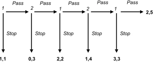
10 Centipede game . . . 45
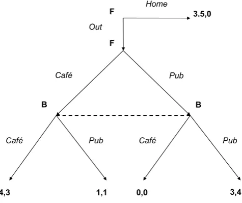
11 Coordination game with an outside option . . . 47
12 Convex hull for the prisoners’ dilemma . . . 60
13 Set of attainable payoffs in the prisoners’ dilemma . . . 61
14 Poor regulatory oversight (c) Scott Adams . . . 65
15 The graphical derivation of the first best outcome . . . 70
16 The graphical derivation of the second best outcome . . . 73
17 Two lotteries and indifference curves in the Marschak-Machina triangle . . . 88
18 Extensive form game for exercise 3, Game Theory 1 . . . 92
19 Extensive form game for exercise 4, Game Theory 1 . . . 92
20 Extensive form game for exercise 5, Game Theory 1 . . . 93
21 Extensive form game for exercise 1, Game Theory 2 . . . 94
22 Range of possible MSNEs in Exercise 2, Game Theory 1 . . . 108
23 Range of possible MSNEs in Exercise 5, Game Theory 1 . . . 112
24 Extensive form game in Exercise 1, Game Theory 2 . . . 116
25 Extensive form game in Exercise 2, Game Theory 2 . . . 118
26 Extensive form game in Exercise 3, Game Theory 2 . . . 120
27 Extensive form game in variant of Exercise 1, Game Theory 2 . . 121
28 First best solution in Exercise 3, Incentive Theory . . . 124
29 Outcome of the first best contracts under asymmetric information in Exercise 3, Incentive Theory . . . 125
30 Second best solution in Exercise 3, Incentive Theory . . . 126
31 First best solution in Exercise 4, Incentive Theory . . . 128
9
Part I
3 INTRODUCTION 10
3
Introduction
This section will give tools to think about choice under uncertainty. A model of behavior when faced with choices among risky lotteries will be presented – The von Neumann-Morgenstern (“vNM”) Expected Utility Theory (“EUT”) (1944).1 The consequences of EUT in terms of prescribed or predicted behavior will be analyzed, and this will be compared with empirical and experimental data on the behavior of agents. That data will be shown not to conform with EUT in some cases, which means EUT may not be an adequate descriptive model of behavior. Alternative models that take better account of the reality of the patterns of decision making of economic agents will thus be presented and discussed.
4
Readings
4.1
Textbook Readings
• Kreps, Ch. 3
• Varian, Ch. 11
• Mas-Colell, Ch. 6.
4.2
Other general readings
The following are useful survey papers, though note that they partly overlap:
• Machina M., 1987, Choice under uncertainty: problems solved and un-solved, Journal of Economic Perspectives 1(1), 121-154.
• Starmer C., 2000, Developments in Non-Expected Utility Theory: The Hunt for a Descriptive Theory of Choice Under Risk, Journal of Economic Literature 38(2), 332-382.
The following website at The Economics New School is well designed and infor-mative:
• Choice under risk and uncertainty, http://cepa.newschool.edu/het/essays/uncert/choicecont.htm The following articles are well written and motivating:
• Chakrabortty A., Why we buy what we buy, The Guardian, May 20th 2008.
• Do economists need brains?, The Economist, July 24th 2008.
1
5 BASIC TOOLS AND NOTATIONS 11
4.3
Articles
2• Bateman I.J., A. Munro, B. Rhodes, C. Starmer and R. Sugden, 1997, A Test of the Theory of Reference Dependent Preferences, Quarterly Journal of Economics 112(2), 479-505.
• Camerer C., 1995, Individual Decision-Making, in J.H. Kagel and A. Roth, Handbook of Experimental Economics, Princeton University Press, Ch. 8, esp. pp. 617-65.
• Hey J. and C. Orme, 1994, Investigating Generalizations Of Expected Utility-Theory Using Experimental-Data, Econometrica 62(6), 1291-1326.
• Kahneman D. and A. Tversky, 1979, Prospect theory: an analysis of de-cision under risk, Econometrica 47(2), 263-291.
• Kahneman D. and A. Tversky, 1999, Choices, values and Frames, Cam-bridge University Press.
• Machina M., 1982, Expected Utility analysis without the independence axiom, Econometrica 50, 277-323.
• Rabin M., 2000, Risk Aversion and Expected-Utility Theory: A Calibra-tion Theorem, Econometrica 68(5), 1281-1292.
• Shefrin H. and M. Statman, 1985, The Disposition to Sell Winners Too Early and Ride Losers Too Long - Theory and Evidence, Journal of Fi-nance 40(3), 777-790.
• Shogren J.F., S.Y. Shin, D.J. Hayes and J.B. Kliebenstein, 1994, Resolv-ing differences in willResolv-ingness to pay and willResolv-ingness to accept, American Economic Review 84(1), 255-270.
• Sugden R., 1985, New developments in the theory of choice under uncer-tainty, Bulletin of Economic Research 38(1), 1-24.
• Sugden R., 2002, Alternatives to Expected Utility: Foundations, in P.J. Hammond, S. Barberá and C. Seidl (eds.), Handbook of Utility Theory Vol. II, Kluwer: Boston.
• Tversky A. and D. Kahneman, 1991, Loss aversion and riskless choice: a reference dependent model, Quarterly Journal of Economics 106(4), 1039-1061.
5
Basic tools and notations
5.1
The objects of preference and choice
‘Lotteries’ or ‘gambles’ or ‘prospects’ are situations where theoutcomeof one’s
actionareuncertain.
2
5 BASIC TOOLS AND NOTATIONS 12
Actions can consist in buying, selling, going out, staying in, buying an um-brella, etc.
Uncertainty may be due to the incomplete information about the action of others, the inability to predict complex events (weather), limitations in one’s capacity to process complex data, etc.
Outcomes are defined in terms of utility. Outcomes will be influenced by your choice of action and the realization of random events on which you have no influence. For example, a chicken that decides to cross a road will either die if a car happens to come by, or live if no car happens to come by. We assign ‘utility’ to those two possible outcomes. At its most basic, utility is defined in terms of preferences, for example, do you prefer sun or rain?
The agent is supposed to know what acts she can choose, i.e. she knows her options. She is also supposed to know the set of all possible ‘state of nature’ that may prevail, as well as be able to evaluate the probability, objective or subjective, of the occurrence of each possible state of nature. She is also sup-posed to be able to evaluate the utility of all possible consequences of each of her actions (outcomes). Consequence functions are defined as what happens if you chose an act and such or such state of nature occurred.
Consider for example a chicken faced with the decision whether to cross the road. The consequence function of crossing the road combined with the event that a car is on the road is what happens in that case, i.e. the chicken is run over and dies. This can be denoted as follows:
c(car on the road
| {z },
event
cross the road
| {z }
action
) = death | {z }
outcome
Under this setting, you are supposed to know the utility of the outcome of your whole set of action under any possible circumstances, e.g. the chicken is supposed to be able to anticipate any possible event that may occur when he crosses the road, and the outcome of his action under any of those events. You know this in advance even though you may never have experienced such combination of circumstances.
Obviously, your choice would be greatly simplified if a function allowed you to calculate the expected utility of an action based on the expected probability of the outcomes that will result from that action and an evaluation of the utility of each of those outcomes, so as to obtain automatically your expected utility from an action.
Why would you want to predict the utility of an action? This is because you are constantly having to make decisions under uncertainty, and want to take the decision that will maximize utility. We will see in the following that subject to some assumptions on how you make basic decisions and rank the utility of events, then one obtain a very simple way to evaluate the utility of any outcome. Let us first present what is a lottery and how they can be represented graphically.
5.2
Lotteries
5 BASIC TOOLS AND NOTATIONS 13
other (e.g. a trip to the moon or a teddy bear).
1. Consider one agent A,for example, agentAis ‘chicken’.
2. (1, ..., s, ..., S)is the set of states of nature, for example (car on the road, no car on the road)
3. (1, ..., x, ..., X)is the set of actions that are available to you, for example (cross the street, don’t cross the street)
4. c(s, x)is a consequence function or outcomes, which is dependend both on the state of naturesand your action x. For example, c(car on the road, cross the street)is ‘death’, as explained above.
5. p(s)is a probability function, that gives out the probability of each state of nature. For example,p(car on the road) = 0.7.
6. Most of the time, one will take action x as given and denote c(s, x) in short hand as cs and p(s) as ps. Then, the lottery L that results from
actionxis defined by the vector C = (c1, ..., cs, ..., cS)of possible
conse-quences of xand its vector P = (p1, ..., ps, ..., pS)of the probabilities of
each consequences inC.
7. Most of the time, one will take the set of consequences as a given, so that lottery L will be denoted by its vector P of probabilities associated to each consequences.
8. Take the set of consequences C = ( death, life on this side of the road, life on the other side of the road). ConsiderL1 the lottery which results
from the action ‘cross the street’ and L2 the lottery which results from
the action ‘don’t cross the street’. In short-hand, one can denote L1 as
(0.7,0,0.3)andL2 as(0,1,0).
(a) If the chicken prefers lotteryL1toL2,one will denote this asL1≻L2
and this guarantees the chicken crosses the road.
(b) If the chicken is indifferent between lottery L1 and lotteryL2, one
will denote this as L1 ∼L2, and the chicken may or may not cross
the road.
(c) If the chicken considers the lotteryL1 to be at least as good asL2,
one will denote this as L1 L2 and say that the chicken has a
weak preference forL1. In that case, one does not know whether the
chicken is indifferent between L1 andL2 or if it actually prefersL1
overL2. One knows however that the chicken does not preferL2over
L1. From an observational point of view, if the chicken crosses the
road, one knows thatL1L2 but nothing more.
9. If the chicken crosses the road, then that means thatL1L2 . However,
saying that L1 L2 does not give any explanation for the behavior of
5 BASIC TOOLS AND NOTATIONS 14
Figure 1: Why did the chicken cross the road? (c) Wiley Miller
5.3
The Marschak-Machina Triangle
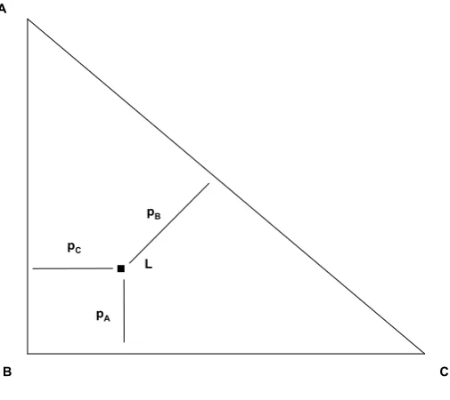
Denote C ={A, B, C} a set of consequences and P = (pA, pB, pC)a vector of
probability defined over C.Note that one will always have pA+pB+pC = 1,
as an event will always occur (‘no event’ is itself an event...). The set P of all possible vectors of probabilities is depicted below in the Marschak-Machina Triangle (‘M-M Triangle’).3
pA
B A
C
.
L pCpB
Figure 2: The Marschak-Machina Triangle
3
[image:15.595.175.428.407.632.2]6 EXPECTED UTILITY THEORY 15
The corners represent the certainty cases, i.e. A is such thatpA= 1, Bis such
that pB = 1andC is such thatpC= 1. A particular lottery,L= (pA, pB, pC)
is represented as a point in the triangle. By convention, cA ≻cB ≻ cC : the
top corner is preferred to the origin which is preferred to the right corner. Any lottery over three events can be represented. pA is measured along the vertical
axis,pC is measured along the horizontal, leavingpB to be measured from the
other vertex. Thus at the origin,B, wherepA andpB are both equal to0, then
pB = 1. The hypotenuse is the range of lotteries for which pB = 0, i.e. the
hypotenuse is all lotteries that combine outcomeAandC only.
We will be interested in the shape of utility indifference curves, which connect all lotteries over which the agent is indifferent. The Marschak-Machina triangle will allow us to show utility indifference curves in a probability space, represented by the triangle. The representation of lotteries in the Marschak-Machina triangle, as well as the representation of preferences over lotteries in this same M-M triangle, will repeatedly be used to illustrate theoretical proposition introduced in those lectures.
Exercises:
1. Represent the following three lotteries in the M-M triangle: L1 =
(0,1,0), L2= (0.5,0,0.5), L3= (1/3,1/3,1/3)
2. Represent the lotteries the chicken is facing when crossing the road, assuming the ordered set of consequences is (death, life on this side of the road, life on the other side of the road) and the probability a car is on the road is0.7.
3. Represent one possible utility indifference curve representing the pref-erences of the chicken if it is found to cross the road. What properties must the utility indifference curve have?
6
Expected Utility Theory
6.1
The axioms of von Neumann and Morgenstern’s
Ex-pected Utility Theory
von Neumann and Morgenstern (“vNM”) Expected Utility Theory (“EUT”) offers four axioms that together will guarantee that preferences over lotteries can be represented through a simple utility functional form.
6.1.1 Completeness
6 EXPECTED UTILITY THEORY 16
This axiom guarantees that preferences are defined over the whole set of possible lotteries. Graphically, in the M-M triangle, this axiom guarantees that any two points in the triangle are either on the same indifference curve or on two differ-ent curves. Indeed, according to the axiom, either the consumer is indifferdiffer-ent between L1 and L2, in which case both lotteries are on the same indifference
curve, or they have a strict preference over L1 and L2,in which case they are
on different indifference curves.
6.1.2 Transitivity
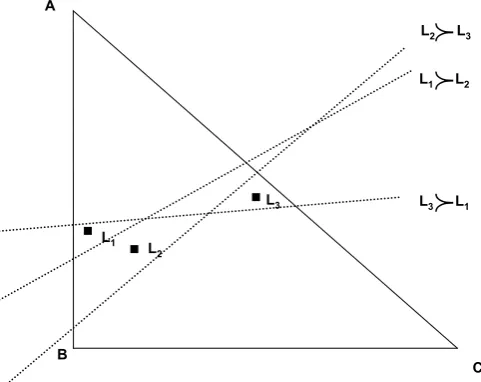
Transitivity axiom: For anyL1, L2, L3,ifL1L2 andL2L3thenL1L3
This axiom guarantees there are no cycles in preferences, i.e. a situation where I prefer bananas to apple, apple to oranges and oranges to bananas is not pos-sible... Graphically, this axiom guarantees that indifference curves in the M-M triangle do not cross. Indeed, if there is intransitivity, then indifference curves must cross inside the triangle. For example, below, I represent indifference curves such thatL1≻L2 andL2≻L3 (note that crossing outside the triangle
is not a problem). Now, you can check that if I want to represent an indifference curve such that L3 ≻L1 (which is intransitive), then it must cross one or the
other or both of the two previous indifference curves inside the triangle (Figure below). Conversely, if indifference curves cross inside the triangle, then there may be situations where transitivity does not hold.
A
C B
.
.
.
L1 L2
L3
L1 L2
f
L3 L1
f
L2 L3
[image:17.595.166.407.453.644.2]f
6 EXPECTED UTILITY THEORY 17
6.1.3 Continuity or Archimedean axiom
Continuity axiom: For anyL3≻L2≻L1,
there exists a uniqueα,0≤α≤1such that αL3+ (1−α)L1∼L2.
Uniqueness ofαguarantees the indifference curves are continuous. This is be-cause this axiom guarantees that any point in the triangle (any lottery) has an equivalent along the hypotenuse, and that this equivalent is unique. Suppose indeed thatL3is the top corner of the triangle andL1the right corner of the
M-M triangle, and considerL2 any point in the triangle. The axiom says that for
someαin[0,1],L2will be equivalent in terms of preferences toαL3+ (1−α)L1
. ButαL3+ (1−α)L1is a point on the hypotenuse of the triangle. Therefore,
any lottery has an equivalent along the hypotenuse, and conversely. This means that there are no spaces either on the hypotenuse or in the triangle that would have no equivalent (there are no ‘jump’ in the indifference curves).
6.1.4 Substitutability or Independence Axiom
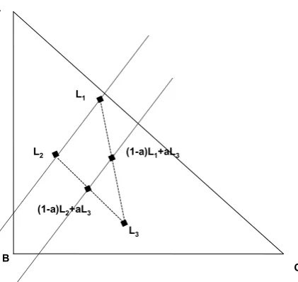
Independence axiom: For anyL1, L2 andL3such that L1≻L2,then
for anyα∈(0,1),(1−α)L1+αL3≻(1−α)L2+αL3.
The independence axiom guarantees that indifference curves are parallel straight lines in the M-M triangle. Indeed, representL1, L2 and L3,three lotteries, in
the M-M triangle. (1−α)L1+αL3and(1−α)L2+αL3are parallel translations
ofL1andL2into the M-M space, so a line that linksL1andL2will be parallel
to a line that links(1−α)L1+αL3and(1−α)L2+αL3. SupposeL1∼L2then
I must have(1−α)L1+αL3∼(1−α)L2+αL3.Therefore, indifference curves
will be parallel across the whole of the triangle (it is just a matter of choosing
6 EXPECTED UTILITY THEORY 18
A
C B
.
.
.
L1
L2
L3
.
.
(1-a)L1+aL3 [image:19.595.197.408.145.344.2](1-a)L2+aL3
Figure 4: Independence axiom
Exercise: The following exercise adresses a common misconception over what
independence means. Suppose you are in Sydney and you are offered lotteries over the outcome spaceC=(train ticket to Paris, train ticket to London). Do you preferp= (1,0)orq= (0,1),i.e. a ticket to Paris or a ticket to London? Suppose now the outcome space isC=(ticket to Paris, ticket to London, movie about Paris). Do you prefer p′ = (0.8,0,0.2)or
q′= (0,0.8,0.2)?
Answer: Many students who say they prefer p to q will also say they prefer
q′ to p′. It may be that this type of choice is the result of improper
understanding of what is a lottery rather than something more basic, so agents do not wantp′ because “there is no point watching a movie about
Paris if I go there anyway”. Indeed, students may not understand that each lottery will result in only one of the outcomes being realized, not two combined outcomes together. An alternative explanation may be that students do not want to face, underp′, the prospect of watching a movie
6 EXPECTED UTILITY THEORY 19
6.2
A Representation Theorem
Theorem 1. [Representation theorem] If the four axioms presented above hold, then there exists a utility indexusuch that ranking according to expected utility accords with actual preference over lotteries. In other words, if we compare two lotteries,L1 andL2 represented by the probability vectors P = (ps)s=1,...,S and
Q= (qs)s=1,...,S over the same set of outcomes S= (1, ..., S)then
L1L2⇔
s=S X
s=1
psu(cs)≤ s=S X
s=1
qsu(cs)
Proof: See pp.176-178 of the Mas-Colell or p. 76 of Kreps. The easiest proof assumes there exist a worst,w,and a best lottery,t,and defines the utility of any lotterypas the number such thatp∼u(p)t+ (1−u(p))w.By con-tinuity, that number exists and is unique. pitself is defined over the set of consequenceC : (a, b, c), and each of those consequences can be ascribed an utility according to the above method. Define thus u(a) the utility of consequencea for example. We havep∼p(a)a+p(b)b+p(c)c(by re-ducibility). We havea∼u(a)t+(1−u(a))w, and similarlybandc. By the independence axiom,p∼(p(a)u(a)+p(b)u(b)+p(c)u(c))t+(1−p(a)u(a)−
p(b)u(b)−p(c)u(c))w.Therefore,u(p) =p(a)u(a) +p(b)u(b) +p(c)u(c).
Notes and implications:
• The utility function is an ordinal measure of utility, not a cardinal measure. This means the specific valueu(cs)is not what is important, rather it is
the ranking of lotteries which must be translated in a correct way by the utility function. This means you do NOT have to translate outcomes into one common measure, such as for example money.
• Said in another way, the theorem is arepresentation theorem – in other words it means we can represent preferences using the utility function, but that doesn’t mean that individuals gain ‘utility’ from outcomes.
• To make the point further, u(.) is unique only up to a positive, linear transformation. This means thatu(.)and any U(.) =a+bu(.)such that
b > 0 represent the same utility function. This means utility numbers have no meaning per se.
• This utility functional has a long history dating back to Bernouilli. The contribution of vNM was to show this was the only type of utility func-tional that respected the above series of four normatively reasonable ax-ioms.
• EU is linear in probabilities. vNM’s EUT makes it possible to obtain preferences between complex lotteries through a simple adding up of the utility of each of the components of the lottery weighted by their respective probabilities.
6 EXPECTED UTILITY THEORY 20
Summing up, one had to remember the following points:
• Axioms of EUT are intuitively ‘reasonable’ assumptions about preferences. Whether they fit real choice (positive axioms) or are good guides for action (normative axioms) is up to one’s perspective. The axioms, while reason-able, are not necessarily prescriptive or necessarily backed up or drawn from experimental evidence. One will see indeed that agent’s actions do not necessarily fit with EUT, which means one or more of the axioms are not respected.
• Together, the axioms imply EUT while EU representations imply the ax-ioms are verified.
• You need to know, understand and be able to use the axioms.
Application to lottery comparisons
EUT provides a simple ways to compare lotteries. Indeed, consider the EU of lotteryLoverx1, x2 andx3:
EU(L) =p1U(x1) +p2U(x2) +p3U(x3) (1)
Rewrite this as
EU(L) =p1U(x1) + (1−p1−p3)U(x2) +p3U(x3) (2)
If we differentiate that equation with respect to probability, then we obtain
dEU(L) =−dp1(U(x2)−U(x1)) +dp3(U(x3)−U(x2) = 0 (3)
for any two points on the same indifference curve. Rearranging,
U(x2)−U(x1)
U(x3)−U(x2)
= dp3
dp1
(4)
which is a constant (check indeed that the ratio is independent of the specific normalization chosen for the utility functional). Therefore, dp3
dp1, which is the slope of indifference lines in the M-M triangle, is always the same, no matter where we are in the Marschak-Machina triangle. This means that once we have found two points in the M-M triangle which give the same utility to a particular person, then we can predict how that person will choose between any two point in the M-M triangle. It is this remarkable feature of expected utility theory which makes it so straightforward to test: you need only find two (non-degenerate) indifferent lotteries to know the preferences over the whole set of lotteries.
7 CRITIQUE OF THE AXIOMS OF EUT 21
Application to risk
Consider an agent with wealth $10,000 and utility normalized to u($x)=ln(x) de-fined over monetary outcomes, i.e. for example, $10 provides utility u($10)=ln(10) = 2.3026.Suppose this agent is offered a lottery(1/2,1/2) over the set of conse-quences (-$100,$101). Will the agent accept the bet?
• If the agent prefers not betting and keeping her $10,000, she gets utility
ln(10000) = 9.2103404.
• If she bets, then she loses $100 with probability 1/2 and gains $101 with probability 1/2, so her expected utility is 1/2 ln(10000−100) + 1/2 ln(10000 + 101) = 9.2103399.
• This is less thanln(10000),so the agent rejects the bet. So far, so good.
• Now, suppose the agent is offered a lottery(1/2,1/2)over the set of conse-quences (-$800,$869). Then you can check she rejects this as well. Indeed,
ln(10000) = 9.2103404 < 1/2 ln(10000−800) + 1/2 ln(10000 + 869) = 9.2103144.
• Suppose now she is offered a lottery(1/2,1/2)over the set of consequences (-$8000,$38476). Then she rejects this as well. Indeed, ln(10000) = 9.2103404<1/2 ln(10000−8000) + 1/2 ln(10000 + 38476) = 9.1948633. Is this reasonable? For more on this issue, read Rabin (2000).4
7
Critique of the axioms of EUT
7.1
The Allais Paradox and fanning out
The Allais paradox (1953)5 was first expressed in the context of the common
ratioeffect, and was then generalized to include thecommon consequenceseffect.
7.1.1 The common ratio effect
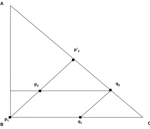
Consider the quartet of distributions(p1, p2, q1, q2)depicted below in a
Marschak-Machina triangle and which, when connected, form a parallelogram. Let them be defined over outcomes (consequences)x1= $0, x2= $50andx3= $100.
1. p1 is (0%,100%,0%): : $0 with 0% chance, $50 with 100% chance, $100
with 0% chance.
4
Rabin M., 2000, Risk Aversion and Expected-Utility Theory, Econometrica 68(5), 1281-1292.
5
7 CRITIQUE OF THE AXIOMS OF EUT 22
2. p2is(1%,89%,10%): $0 with 1% chance, $50 with 89% chance, $100 with
10% chance.
3. q1 = (89%,11%,0%): $0 with 89% chance, $50 with 11% chance, $100
with 0% chance.
4. q2 = (90%,0%,10%): : $0 with 90% chance, $50 with 0% chance, $100
with 10% chance.
When confronted with this set of lotteries, there are people who choosep1 over
p2and chooseq2overq1. This contradicts the independence axiom of expected
utility, as we are going to prove, both diagrammatically and analytically, that an expected utility maximizer who prefersp1top2ought to preferq1toq2.This
contradiction is called the “Allais Paradox”.
Diagram (see figure below): Consider the diagram below where the four lot-teries above are represented. Note how the line that connectsp1 andp2,
and the one that connects q1 and q2, are parallel. If indifference curves
are parallel to each other, as in EUT, then it should be if p1 ≻ p2 then
q1≻q2. We can see this diagrammatically by considering an indifference
curve which translates the fact thatp1≻p2: it ought to separatep1from
p2, withp1 above andp2 below. A parallel indifference curve will divide
q1fromq2, withq1above andq2below, from which one can conclude that
q1≻q2.
A
C
.
p2
.
.
.
p1
.
p’2
q1
q2
[image:23.595.173.426.441.659.2]B
7 CRITIQUE OF THE AXIOMS OF EUT 23
Analysis: An analytical proof would go as follows: Asp1 ≻ p2 then by the
von Neumann-Morgenstern expected utility representation, there is some elementary utility functionusuch that:
u($50)>0.1u($100) + 0.89u($50) + 0.01u($0) (5)
But as we can decompose
u($50) = 0.1u($50) + 0.89u($50) + 0.01u($50) (6) then subtracting0.89u($50)from both sides, the first equation implies:
0.1u($50) + 0.01u($50)>0.1u($100) + 0.01u($0) (7)
Adding0.89u($0)to both sides:
0.1u($50) + 0.01u($50) + 0.89u($0)>0.1u($100) + 0.01u($0) + 0.89u($0)
(8) Combining the similar terms together, this means:
0.11u($50) + 0.89u($0)>0.1u($100) + 0.90u(0) (9)
which implies thatq1≻q2, which is what we sought.
7.1.2 The common consequence effect.
With reference to the graph above, tests of the common ratio effect involve pairs of choices like(p1orp2)and(q1orq2). Tests of the common consequence effect
involve pairs of choices like(p1 orp′2)and(q1or q2).
Example: Consider the choice betweenp1= (0%,100%,0%)andp′2= (9%,0%,91%).
Suppose the agent prefersp1 top′2 but prefersq2 to q1. Graphically, one
can see that this contradicts the independence axiom too.
The ‘common consequence’ effect is less robust than the ‘common ratio’ effect, i.e. the contradiction in choice is less often observed in that case. This may be due to the simpler nature of common consequences lotteries, which as the name indicates involve comparison between lotteries defined across a maximum of two consequences only, rather than a maximum of three in the common ratio effect. Part of the issue with the common ratio effect may thus be due to how complicated that type of choice is, rather than to some inherent behavior pattern.
7.2
Process violation
A common example of violation of transitivity is the “P-bet, $-bet” problem:
7 CRITIQUE OF THE AXIOMS OF EUT 24
1. P-bet: $30 with 90% probability, and zero otherwise.
2. $-bet: $100 with 30% probability and zero otherwise.
An agent is first asked which lottery they would prefer playing, and then asked what price they would buy a ticket to play the P-bet or the $-bet. Notice that in this example, the expected payoff of the $-bet is higher than that of P-bet, but the $-bet is also more risky (lower probability to win). This may be why people tend to choose to play the P-bet over the $-bet. Yet, the same people are ready to paymore for a ticket to play the $-bet than for a ticket to play a P-bet. Said in another way, although when directly asked, they would choose the P-bet, they are willing to pay a lower certainty-equivalent amount of money for a P-bet than they do for a $-bet. For example, they might express a preference for the P-bet, but be ready only to pay $25 to play the P-bet while being ready to pay $27 for the $-bet.
Many have claimed that this violates the transitivity axiom. The argument is that one must be indifferent between the certainty-equivalent amount (“price”) of the bet and playing it, so that in utility terms, taking the example above again, I would haveU(P−bet) =U($25)andU($−bet) =U($27). By monotonicity, since more money is better than less money,U($27)> U($25)and so we should conclude thatU($−bet)> U(P−bet). Yet, when asked directly, people usually prefer theP−betto the$−bet, implyingU(P−bet)> U($−bet).Thus, the intransitivity.
However, the question is whether this “intransitivity” is not simply due to overpricing of $-bets, i.e. agents being unable to price bets correctly. For example, I once offered to a student a ticket for a bet giving 12 chance of $100 and 12 chance of $0. I was offered $12 in exchange for that ticket. When I asked the same person how much they would sell me a ticket for this bet, they quoted a price of $43... Was the discrepancy due to improper understanding by the student, to lack of experience, to an exaggerated fear of getting it “wrong” in front of others, or to the fact this was not real money? Would the discrepancy have survived if the student had been given the opportunity to change his bids, or if a negotiation process had been put in place? One could design a series of alternative design for the experiment, but it illustrates a Willingness to Accept / Willingness to Pay disparity that survives whatever the experimental set-up (on the discrepancy WTA/WTP, see ‘endowment effect’)
7.3
Framing effect and elicitation bias
In order to determine if the P-bet, $-bet anomaly is due to the procedure by which the preference between lotteries is elicited, or to true intransitivity in preferences, consider an experiment mentioned by Camerer (1995).6 In this experiment, the P-bet offers $4 with probability 35
36, 0 else, while the $-bet
offers $16 with probability 11
36,0 else.
The subject is asked to choose between the two, and then is asked how much they are prepared to pay for each of them:
6
7 CRITIQUE OF THE AXIOMS OF EUT 25
• If the subject chose the P-bet and quoted a higher price (e.g. $3.5) for it than for the $-bet (e.g. $3), then the preferences were judged to be coherent.
• If the subject chose the P-bet but then quoted a lower price (e.g. $3.5) for it than for the $-bet (e.g. $4.5), then this was judged to potentially indicate a reversal of preference. In order to determine if that potential reversal was merely due to overpricing of the $-bet, experimenters then asked the subject to choose between each bet and a stated amount, $4 in this case.
– If the subject chooses $4 rather than the $-bet, then that means they previously overpriced the $-bet and there was thus a framing effect at play rather than a true violation of transitivity. Indeed, the only reason there was an apparent violation of transitivity is merely that in one case the subject was asked to make a choice between lotteries, and in the second case, he was asked to price lotteries. Those are rather different mental processes.
– If on the other hand the subject indeed choose the $-bet over the $4 and the $4 over the P-bet, then that meant there was true violation of transitivity, independent of any framing effect. Indeed, the ques-tion was framed the same way (choice between lotteries) and led to a contradiction of transitivity.
Loomes, Starmer and Sugden (1991)7 contend that violations of transitivity may occur because agents use rather less sophisticated techniques than EUT to evaluate lotteries. They posit that agents tend to choose lotteries with the larger probability as long as the payoffs are close, and choose lotteries with the larger payoff is the payoffs are far away. This can lead to intransivities. For example, suppose an agent is asked to choose between 60% probability of get-ting $8(L1)and 30% probability of getting $18(L2). Payoffs are close, so most
agents choose the first as it has higher probabilities to win. Suppose then the agent is offered $4 for sure against 60% probability of getting $8. Again, payoffs are close, so most people agents choose the first. Finally, however, most agents would choose 30% probability of getting $18 rather than $4 with certainty, as payoffs are far apart so the lottery with the higher payoff is preferred. This leads to a violation of transitivity. Indeed, the first choice impliesu(L1)> u(L2).The
second choice implies u(L1)< u($4). The third choice impliesu(L2)> u($4).
Combining the two last choices, u(L2)> u(L1),which contradicts the original
choice between lotteries. As above, the advantage of this design is that the agent is always asked for their choice among lotteries and are never asked to evaluate them individually.
This can be generalized to say that agents will try to minimize the number of informations on which to draw their decisions rather than taking into account all the parameters in the decision. E.g. when choosing between two brands
7
7 CRITIQUE OF THE AXIOMS OF EUT 26
of foods, you will not look all the ingredients that came into their making but rather will choose salient dimensions such as sugar content and price to make your decision. For a very interesting account of the kind of reasoning people do when buying, see Viswanathan, Rosa and Harris (2005).8 For more on de-signing experiments to avoid ‘framing’ subjects, i.e. to avoid obtaining results that are dependent on the design on the experiment rather than on true subject behavior, read Machina (1987).9
7.4
Endowment effects
The endowment effect is such that people are less willing to pay for an object than they would ask as payment if they owned it. This is the difference between the WTP (Willingness To Pay) and the WTA (Willingness To Accept). This ‘endowment effects’ is not explained by wealth effects, but may be due to loss aversion (which will come up in ‘regret theory’). For example, if losses are more painful than equally sized gains are pleasurable, then one will offer to pay only $12 to play a lottery with 50% chance of getting $100 so as to minimize loss in case of bad luck (when the lottery draws $0, so the loss is $12), while one will be prepared to sell the bet only at the much higher $43 to minimize loss in case of bad luck, in this case, when the lottery draws $100 (the loss is $57).
Note that the disparity between WTP and WTA is explained in some measure within EUT, but not to the extent it appears in reality. For more on this, see exercise 5 of Choice under Uncertainty.
7.5
Discussion
Those experiments that contradict the predictions of EUT are interesting be-cause they do not require to estimate utility functions for individuals, and they allow for a direct test of the axioms. The drawback is that they do not allow one to know how ‘badly’ inconsistent the choices of the agents are. This would require many more experiments. The only information from those experiments is the percentage of individuals whose choices violate EUT, and in what specific way the choice is violated. An obvious critique of the above experiments is that the choices asked from subjects in those experiments are rather too complicated and unintuitive compared with the type of choices they are facing in real life. The issue is then to present the problem in an intuitive form, or to allow the subjects to get acquainted with the way the experiment is set up and the way its consequences will affect them (i.e. let them play many rounds).
Note however that some of the experiments exposed above were adapted to rats using food as a currency and those experiments showed violations of the independence axiom as well. This points to a possible evolutionary benefit of
8
Viswanathan M., J.A. Rosa and J.E. Harris, 2005, Decision Making and Coping of Func-tionally Illiterate Consumers and Some Implications for Marketing, Journal of Marketing 69(1), 15-31.
9
8 ALTERNATIVES AND GENERALIZATIONS OF EUT 27
behaving in ways that are different from those of an expected utility maximizer. Some experiments have been done comparing how farmers in traditional farming communities evaluate lotteries, and have indeed shown their behavior, while different from urbanized people, may have evolutionary benefits in a context where droughts and famines are likely (Humphrey and Verschoor (2004).10
8
Alternatives and generalizations of EUT
Contradictions within the framework of EUT led to the development of various alternatives to EUT, of which we will present some. In a first part, we consider prospect theory and its successors, in a second part we consider regret theory. Starmer (2000)11provides good further reading on this topic.
8.1
Prospect Theory, Rank Dependent EUT and
Cumu-lative Prospect Theory
In this section, by order of difficulty and chronology, we consider prospect the-ory (‘PT’) by Kahneman and Tversky (1979),12 rank dependent utility theory (‘RDEUT’) (Quiggin, 1982),13and Cumulative Prospect Theory (‘CPT’) (Kah-neman and Tversky, 1992).14 Those utility representations differ from EUT by considering subjective probabilities as a function of objective probabilities, that correspond to how people estimate probabilities in reality (probability weighting functions). They also differ by considering an “editing phase”, whereby one di-vides the set of consequences of a lottery into either ‘gains’ or ‘losses’. Different probability weighting functions are assigned to probabilities of a consequence depending on whether the consequence is a gain or a loss.
8.1.1 Prospect Theory
Consider the set of consequences C = (a, b, c, d) such thata≺b ≺c ≺d and consider lottery L = (pa, pb, pc, pd). Under prospect theory, its utility function
is of the form:
U(L) =π(pa)u(a) +π(pb)u(b) +π(pc)u(c) +π(pd)u(d) (10)
π(p), the probability weighting function, takes the following form:
10
Humphrey S.J. and A. Verschoor, 2004, Decision-making Under Risk among Small Farm-ers in East Uganda, Journal of African Economies 13(1), 44-101.
11
Starmer C., 2000, Developments in Non-expected Utility Theory: The Hunt for a De-scriptive Theory of Choice under Risk, Journal of Economic Literature 38(2), 332-382.
12
Kahneman D. and A. Tversky, 1979, Prospect Theory: An Analysis of Decision under Risk, Econometrica 47(2), 263-291.
13
Quiggin J.C., 1982, A theory of anticipated utility, Journal of Economic Behavior and Uncertainty 3(4), 323-343.
14
8 ALTERNATIVES AND GENERALIZATIONS OF EUT 28
p
!(p)
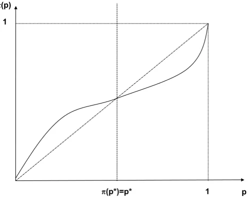
[image:29.595.177.427.149.350.2]!(p*)=p* 1 1
Figure 6: Probability weighting function
The reason for offering that type of representation is that there tends to be a dif-ference between ‘psychological probability’ and ‘objective probability’: agents are quite able to estimate lotteries with probability between around 1/3 and
2/3but overestimate low occurrence events and underestimate high occurrence events. Below p∗ in the graph above, the agent weighs events above their
sta-tistical probability, while this is the opposite for events with stasta-tistical prob-ability above p∗. Intuitively, agents overweigh the probability of events with
low statistical probabilities, maybe because they are not used to estimating the probability of their occurence and they feel anxious about them. The other side of the coin is that they will under-estimate the probability of events that are statistically quasi-given. If for example I over-estimate the probability of being run down by a car (low probability event), then this means I underestimate the probability that I will cross the road safely (high probability event). p∗,which is
the probability that agents are able to estimate correctly, is variously evaluated between0.3and0.5.
8 ALTERNATIVES AND GENERALIZATIONS OF EUT 29
with probability weighting functions. One would thus have:
π(5%)u(100) +π(95%)u(0) =u(6) (11)
π(50%)u(100) +π(50%)u(0) =u(50) (12)
π(95%)u(100) +π(5%)u(0) =u(93) (13) Normalizingu(0) = 0,then one finds that
π(5%) =u(6)/u(100) (14)
π(50%) =u(50)/u(100) (15)
π(95%) =u(93)/u(100) (16)
Suppose the agent is risk neutral, then
π(5%) = 6/100 (17)
π(50%) = 1/2 (18)
π(95%) = 93/100 (19)
CPT thus does not require one to assume anything other than risk-neutrality to explain the pricing of the different lotteries above.
8.1.2 Rank Dependent EUT
RDEUT differs from PT in that it requires that the sum of probabilies over a whole set of events be equal to one. This is doe as follows: If one orders events from the least to the most preferred, ( a ≺ b ≺ c ≺ d), then one writes the utility of lottery L= (pa, pb, pc, pd)as:
U(L) =f(pa)u(a) +f(pb)u(b) +f(pc)u(c) +f(pd)u(d) (20)
with
f(pa) =π(pa) (21)
f(pb) =π(pa+pb)−π(pa) (22)
f(pc) =π(pa+pb+pc)−π(pa+pb) (23)
f(pd) = 1−π(pa+pb+pc) (24)
Compared with PT, RDEUT guarantees that the sum of the probability weights assigned to each events sum up to1. Check indeed thatf(pa) +f(pb) +f(pc) +
f(pd) = 1.In RDEUT,f(.)is a cumulative probability function, with outcomes
added in the order of their preferences.
8.1.3 Cumulative Prospect Theory
8 ALTERNATIVES AND GENERALIZATIONS OF EUT 30
Suppose for example that I consider a and b as losses and c and d as gains. DefiningfG the probability weighting utility function applied to gains, andfL
the probability weighting function applied to losses, I then have
U(L) =fL(pa)u(a) +fL(pb)u(b) +fG(pc)u(c) +fG(pd)u(d) (25)
with
fL(pa) =πL(pa) (26)
fL(pb) =πL(pa+pb)−πL(pa) (27)
fG(pc) =πG(pc+pd)−πG(pd) (28)
fG(pd) =πG(pd) (29)
withπG(.)defined over gains andπL(.)defined over losses, both increasing. In
order to guarantee the sum of probabilies is one as in RDEUT, I must have that
πL(pa+pb) = 1−πG(pc+pd),that is, the cumulative probabilities of loss events
is the complement of the cumulative probabilities of gain events. CPT differs from RDEUT by taking into account whether the event is considered as a loss or as a gain. This is intuitively justified by saying that losses affect the agent more than gains, and are thus overweighted. The distinction between ‘gain’ and ‘losses’ is of course subjective, and must be calibrated depending on the individual and the situation. An alternative way to consider gains and losses is to assign different utility functionals to gains compared to losses, whereby agents are almost risk neutral with respect to gain (for example, a50/50chance to gain
$100 would be evaluated at $49), while being very risk averse with respect to losses (for example, a 50/50chance to lose $100would be evaluated at −$60, i.e. the agent is ready to pay $60not to play the lottery).
8 ALTERNATIVES AND GENERALIZATIONS OF EUT 31
A
C B
U1
U2
[image:32.595.185.411.142.352.2]U3
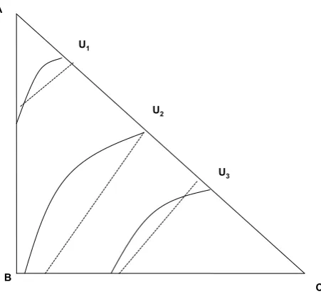
Figure 7: RDEUT and CPT curves
At this point, given the complexity of the arguments, it is rather difficult to make intuitive reasonings to justify the precise shape of the indifference curves. Consider however the indifference curve corresponding to utilityU2.If the agent
was an EU maximizer, then its indifference curve would take the form of the dotted line. On the hypothenuse, one considers a lottery with equal probability betweenAandC,which the agent evaluates as in EUT (if one assumesp∗= 0.5).
On the line joiningBandC,one has a lottery with a better outcome with high probability, which is going to be under-evaluated, which explains the indifference curve is above the EU curve with the corresponding utility. However, the under-evaluation is not so high since the probability of the best event is 0. As the probability of that best event increases, so does the discrepancy, until a point where the discrepancy decreases again as the lotteries involve closer outcomes. The indifference curves are thus concave.
Exercises:
1) Try to justify the compared shape of the EU and RDEU curves at level of utilityU1and level of utilityU3.
2) How does CPT change the shape of the curve compared to RDEUT?
8.2
Regret theory
8 ALTERNATIVES AND GENERALIZATIONS OF EUT 32
a lottery over another and then comparing their outcome is expected to make one happy/unhappy. To the difference of other theories, regret theory explicitly takes into account the opportunity cost of making a decision. Decisions are not taken in a vacuum; making one decision precludes making another one. The theory is exposed in Loomes and Sugden (82, 86)1516 and Sugden (85).17 Agents thus faced with alternative lotteries do not seek to maximize expected utility but rather to minimize expected regret (or maximize expected rejoicing) from their choice.
Formally, suppose lotteryphas probabilities(p1, .., pn)while lotteryq
probabil-ities(q1, .., qn)over the same finite set of outcomes x= (x1, ..., xn). Expected
rejoice/regret from choosingpoverq is:
E(r(p, q)) =X
i X
j
piqjr(xi, xj) (30)
wherepiqjis the probability of outcomexiin lotterypand outcomexjin lottery
qj. Lotterypwill be chosen over lotteryqifE(r(p, q))is positive andqwill be
chosen overpifE(r(p, q))is negative.
Note that ifr(xi, xj) =u(xi)−u(xj)thenE(r(p, q))is simply the difference in
expected utility between lotterypandqand regret theory leads to exactly the same decision as EUT.
Under regret theory:
1. r(x, y)is increasing in xso that the higher the good outcome, the higher the rejoicing.
2. r(x, y) =−r(y, x), so that regret/rejoice is symmetric: Getting the good outcome x rather than the bad outcome y produces the same amount of rejoicing than the amount of regret induced by getting the symmetric outcome. The expected rejoice at a gain is the same as the expected regret at a same sized loss,
3. r(x, y)> r(x, z) +r(z, y)when x > z > y, that is the rejoicing increases more than proportionately with the difference in outcome. I rejoice more if I gain $100 rather than $0 than the sum of rejoicing if I gain $50 rather than $0 and $100 rather than $50, even though the result is the same. Consider for example how French people would react if their rugby team beat Australia (pride, celebration), compared to how they would react if France beat New Zealand (the usual...), and New Zealand beat Australia (no one cares, at least in France, except maybe in Toulouse...).
The advantage of the regret/rejoice model is that the “indifference curves” over lotteries derived from it can be intransitive, i.e. yield up preference reversals. From the beginning of the course, we know that this means indifference curves
15
Loomes G. and R. Sugden, 1982, Regret Theory: An Alternative Theory of Rational Choice Under Uncertainty, The Economic Journal 92(368), 805-824.
16
Loomes G. and R. Sugden, 1986, Disappointment and Dynamic Consistency in Choice under Uncertainty, The Review of Economic Studies 53(2), 271-282.
17
8 ALTERNATIVES AND GENERALIZATIONS OF EUT 33
can cross inside the M-M triangle. Exercise 6 in ‘Choice under Uncertainty’ shows that not only does RT allow for intransitive preferences, but it also man-dates one specific direction in which preferences can be intransitive, i.e. while it would allow A≻B ≻C≻A, it would not allowA≺B≺C≺A. This means that a test of RT is to check that intransitiveness, when it occurs, occurs in one direction only. Experiments tend to bear this out.
34
Part II
Game theory
9 INTRODUCTION 35
9
Introduction
This section aims to present essential tools for predicting players’ actions in a range of strategic situations. By order of complexity, we will study strategic form games, where players choose actions at the same time so there is no con-ditioning of actions based on the action of others, extensive form games where players choose actions in succession but know what action was taken by others previously so there is no uncertainty, and finally Bayesian games where players choose action in succession but are not certain what the other played previously. We will also cover repeated games under full information, where players condi-tion their accondi-tion on their observacondi-tion of what was played in a previous stage of the game.
The lecture builds on the analysis of one single game, a coordination game, which is made progressively more complex so as to introduce new concepts. Those in-clude the concept of dominant strategy, Nash equilibrium, mixed strategy Nash equilibrium, backward induction, subgame perfect Nash equilibrium, Bayesian Nash equilibrium and forward induction. A few other games are introduced, includings games of auctions (to illustrate the use of Bayesian Nash equilibrium concepts) and the Prisoners’ dilemma (in relation to infinitely repeated games).
This lecture does not introduce many applications of game theory, as it is ex-pected the student will encounter applications relevant to his or her area of specialization further on in the course of his or her MSc. Rather, the lecture aims to give good mastery of notations and techniques for solving a wide range of games.
10
Readings:
10.1
Textbook reading:
• Kreps, Chs. 11-14
• Varian, Ch. 15
• Mas-Colell, Chs. 7-9
Among the many specialist text books which are currently available, by degree of difficulty, one finds:
• Carmichael F., 2005, A Guide to Game Theory, FT Prentice Hall (less advanced)
• Gibbons R., 1992, A Primer in Game Theory, FT Prentice Hall (more advanced)
11 STRATEGIC FORM GAMES 36
10.2
Articles
18• Cho I.-K. and D. Kreps, 1987, Signalling Games and Stable Equilibria, Quarterly Journal of Economics 102, 179-222.
• Cho I.-K. and J. Sobel, 1990, Strategic Stability and Uniqueness in Sig-nalling Games, Journal of Economic Theory 50, 381-413.
• Geanakoplos J., 1992, Common Knowledge, The Journal of Economic Perspectives 6, 53-82.
• Goeree J.K. and C.A. Holt, 2001, Ten Little Treasures of Game Theory and Ten Intuitive Contradictions, American Economic Review 91(5), 1402-1422.19
• Mailath G.J., L. Samuelson and M. Swinkels, 1993, Extensive form rea-soning in normal form games, Econometrica 61, 273-302.
• Palacios-Huerta I., 2003, Professionals play minimax, Review Of Economic Studies 70(2), 395-415.
• Rubinstein A., 1991, Comments on the Interpretation of Game Theory, Econometrica 59, 909-924.
• Shaked A., 1982, Existence and Computation of Mixed Strategy Nash Equilibrium for 3-Firms Location Problem, Journal of Industrial Eco-nomics 31, 93-96.
• Van Damme E., 1989, Stable equilibria and forward induction, Journal of Economic Theory 48(2), 476-496.
11
Strategic form games
Definition: A strategic form game is defined by:
1. Players: The set N = 1, ..., i, ..., n of agents who play the game, for example: Adelina and Rocco.
2. Strategies: For eachi∈N, I define the set of strategiesSi with
typi-cal elementsi available to agenti, for example, {Cooperate, Defect}.
3. Payoffs: DenoteS = (S1, ..., Si, ..., Sn)the set of all strategies
avail-able to all the players, for example ({Cooperate, Defect},{Cooperate, Defect}).
To each strategy profiles= (s1, ..., si, ..., sn)inS, for example (Cooperate,
Defect), one associates payoffui(s)corresponding to that combination of
strategies. u= (u1, ..., ui, ..., un)is the set of payoffs of the game, defined
for allsin S.
18
Some articles in this list were contributed by previous teachers in MSc Economic Theory 1 at the UEA.
19
11 STRATEGIC FORM GAMES 37
G=N, S, udefines a strategic form game.
Notation: One will denote s−i = {s1, ..., si−1, si+1, ..., sn} the set of actions
taken by agents other thaniin the strategy profilesandS−i ={S1, ..., Si−1, Si+1, ..., Sn}
the set of strategies available to players other thani. Example: The Prisoners’ Dilemma
1. Players N= 1,2.
2. StrategiesSi=C, D,i= 1,2
3. Payoffs u1(C, D) = u2(D, C) = −6, u1(C, C) = u1(C, C) = −1,
u1(D, C) =u2(C, D) = 0andu1(D, D) =u2(D, D) =−4.
The game can be represented in normal form as follows:
C D
C -1,-1 -6,0
D 0,-6 -4,-4
11.1
Dominance
The following definitions introduce the concept of a strictly dominant strategy equilibrium. In a strictly dominant strategy equilibrium, players play their strategy irrespective of the action of others.
Definition: Strategysi∈Sistrictly dominates strategys′i6=siinSifor player
iifui(si, s−i)> ui(s′i, s−i)for alls−i in S−i.
Ifsistrictly dominates another strategiess′i, then that strategy is strictly
dom-inated and can be elimdom-inated from consideration byi.
Definition: Strategys′
i is strictly dominated if there is ansi∈Si that strictly
dominates it.
If si strictly dominates all other strategies, then it is strictly dominant. Note
that si is by definition unique.
Definition: si∈Si is strictly dominant foriif it strictly dominates alls′i6=si
inSi.
An equilibrium in strictly dominant strategies exists if all players have a strictly dominant strategy. Note that from the above, a strictly dominant strategy is necessarily unique.
Definition: s∗∈S is a strictly dominant strategy equilibrium ifu
i(s∗i, s−i)>
ui(si, s−i)for all playersi∈Nand for all strategy profiless−i ∈S−i,that
11 STRATEGIC FORM GAMES 38
Example: The strictly dominant strategy equilibrium in the Prisoners’ Dilemma is {D,D}. Indeed, D is a strictly dominant strategy for player 1 asu1(D, C)>
u1(C, C)andu1(D, D)> u1(C, D). The same holds for player2.
Remark: One can also define weak dominance as follows: Strategy si ∈ Si
weakly dominates (or simply “dominates”) strategys′
i6=siinSifor player
iifui(si, s−i)≥ui(s′i, s−i)for alls−i in S−i.
11.1.1 Iterated delection of strictly dominated strategies
A strategys′
i that is strictly dominated will not be part of any equilibrium of
the game. One can therefore exclude strictly dominated strategies from the set of available strategies.
Example: Consider the following example:
L M R
U 2,3 4,1 -1,6
D 5,3 4,-5 7,4
M is strictly dominated by L. L is strictly dominated by R. Both L and M can thus be eliminated. U is only weakly dominated by D, as it obtains the same payoff as D when 2 plays M. It cannot thus be eliminated from the set of available strategies.
One obtains the following remaining game:
R U -1,6
D 7,4
In that remaining game, U is strictly dominated by D. The dominant strategy equilibrium of the game, obtained by iterated deletion of strictly dominated strategies, is thus (D, R).
Games with a strictly dominant strategy equilibrium are of limited interest. Indeed, in so far as players’ actions are not dependent on others’ action, those games cannot properly be called strategic. We introduce in the following part a concept, that of Nash equilibrium, which is of interest in proper strategic games.
11.2
Nash equilibrium
Definition: A Nash equilibrium (‘NE’) is a strategy profile s∗ such that for
every playeri,ui(s∗i, s∗−i)≥ui(si, s∗−i)for allsi∈Si.
Note how different the NE concept is from the dominant strategy concept: the NE concept does not require thats∗
i be dominant for alls−i in S−i, but only
fors∗
−i. That is,taking s∗−i as given, agentimust not strictly prefer to deviate
11 STRATEGIC FORM GAMES 39
Example: Nash Equilibrium in a Coordination Game 1. Players N=French (F), British (B).
2. StrategiesSi=Coffee (C), Pub (P), i=F,B
3. Payoffs uF(C, P) = uB(C, P) = 1, uF(C, C) = uB(P, P) = 4,
uF(P, C) =uB(P, C) = 0anduF(P, P) =u2(C, C) = 3.
The game can be represented in normal form as follows:
B
C P
F C 4,3 1,1
P 0,0 3,4
Neither strategies is strictly (or weakly) dominated for either players. However, suppose that F plays C. Then B is better off playing C. Sup-pose that F plays P. Then B is better off playing P. Formally,uF(C, C)≥
uF(P, C)and uB(C, C)≥uB(C, P). Similarly, uF(P, P)≥uF(C, P)and
uB(P, P)≥uB(P, C).This means that both {C, C} and{P, P}are Nash
equilibria of the game.
Note how we found two Nash equilibria of the game above. This generalizes to saying that Nash equilibria are not necessarily unique, unlike dominant strategy equilibria. However, from the definition, one can check that any dominant strat-egy equilibrium is also a Nash equilibrium. There is no way in the game above to choose which of the Nash equilibria is more likely to be chosen. However, the Nash equilibrium concept allows one to say that players will play either one or the other Nash equilibria. The Nash equilibria we found are such that players choose actions in a deterministic way, that is, if for example the Nash equilib-rium is {C,C}, then both players play C. Those are called pure strategy Nash equilibria (‘PSNE’). We will see below there exists a third Nash equilibrium of this game, where players choose actions at random according to pre-defined probability. Those are called mixed stategy Nash equilibria (‘MSNE’).
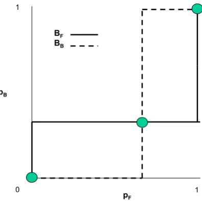
A common way to find Nash equilibria is to use the concept of Best Response Function, which is particularly useful when players’ action set is continuous (such as quantity or price in a game of competition).
Definition: The best-response function (‘BRF’) for player i is a functionBi
such thatBi(s−i) ={si|ui(si, s−i)≥ui(s′i, s−i)for alls′i}.The BRF states
what is the best action forithe whole range of possible profile of actions of other agents.
Definition: s∗ is a Nash equilibrium if and only ifs∗
i ∈Bi(s∗−i)for alli. This
means that elements ofs∗ must be best responses to each other.
Example: In the example above, BF(C) = C and BF(P) = P. Similarly,
11 STRATEGIC FORM GAMES 40
11.2.1 Nash equilibrium in mixed strategies
In the following, we consider the possibility for players to choose actions at random according to pre-defined probabilities. For the sake of easy modeling, we assume agents have access to a randomizing device (such as a coin for example), which allows them to randomize over their actions. For example, an agent who decides to play C with probability 1/8 in the game above can do so by saying he will play C whenever three throws of the coin all give out ‘tail’. We will see later whether agents can randomize in an accurate and rational way without access to such a randomizing device.
Example: Mixed strategy Nash equilibria (‘MSNE’) in the Coordination Game: We did not consider above the case of mixed strategies. Consider thus strategiessi of the form: i plays C with probability pi and playP with
probability 1−pi. Strategy si can be denoted in short as pi. Suppose
players F and B play strategies pF and pB respectively. The payoff to
F of playing C is then uF(C, pB) = 4pB+ 1(1−pB) = 3pB + 1.
Sim-ilarly, uF(P, pB) = 3−3pB. I also obtain that uB(pF, C) = 3pF and
uB(pF, P) =pF+ 4(1−pF) = 4−3pF.
Therefore,F will playC whenever3pB+ 1>3−3pB,that is, whenever
pB >13. She will playP wheneverpB< 13 and will be indifferent between
the two actions whenever pB = 13. Similarly, B will play C whenever
3pF >4−3pF,that is ifpF > 23. He will playP wheneverpF < 23, and
will be indifferent between the two actions wheneverpF = 23.
One thus has three Nash equilibria:{pF = 0, pB= 0}and{pF = 1, pB = 1}
as before, and a mixed strategy Nash Equilibrium 2 3,
1
3 whereby each
player plays its own favorite option with probability 2
3,and the other
op-tion with probability 1
3.Under that MSNE, the payoff forF is2 and the
payoff forB is 2as well.