Munich Personal RePEc Archive
Zenga’s new index of economic
inequality, its estimation, and an analysis
of incomes in Italy
Greselin, Francesca and Pasquazzi, Leo and Zitikis, Ricardas
Dipartimento di Metodi Quantitativi per le Scienze Economiche e
Aziendali„ Dipartimento di Metodi Quantitativi per le Scienze
Economiche e Aziendali„ Department of Statistical and Actuarial
Sciences, University of Western Ontario,
August 2009
Online at
https://mpra.ub.uni-muenchen.de/17147/
ESTIMATION, AND AN ANALYSIS OF INCOMES IN ITALY
Francesca Greselin
Dipartimento di Metodi Quantitativi per le Scienze Economiche e Aziendali, Universit´a di Milano Bicocca, Milan, Italy.
E-mail: francesca.greselin@unimib.it
Leo Pasquazzi
Dipartimento di Metodi Quantitativi per le Scienze Economiche e Aziendali, Universit´a di Milano Bicocca, Milan, Italy. E-mail: leo.pasquazzi@unimib.it
Riˇcardas Zitikis
Department of Statistical and Actuarial Sciences, University of Western Ontario, London, Ontario N6A 5B7, Canada. E-mail: zitikis@stats.uwo.ca
Abstract. For at least a century academics and governmental researchers have been developing measures that would aid them in understanding income distributions, their differences with respect to geographic regions, and changes over time periods. It is a challenging area due to a number of reasons, one of them being the fact that different measures, or indices, are needed to reveal different features of income distributions. Keeping also in mind that the notions of ‘poor’ and ‘rich’ are relative to each other, M. Zenga has recently proposed a new index of economic inequality. The index is remarkably insightful and useful, but deriving statistical inferential results has been a challenge. For example, unlike many other indices, Zenga’s new index does not fall into the classes of L-, U-, and V-statistics. In this paper we derive desired statistical inferential results, explore their performance in a simulation study, and then employ the results to analyze data from the Bank of Italy’sSurvey on Household Income and Wealth.
Keywords and phrases: Zenga index, lower conditional expectation, upper conditional expectation, confidence interval, Bonferroni curve, Lorenz curve, Vervaat process.
1. Introduction
Measuring and analyzing incomes, losses, risks and other (non-negative) random outcomes, which we denote by X, has been an active and fruitful research area, par-ticularly in the fields of econometrics and actuarial science. The Gini index has been arguably the most popular measure of inequality, with a number of extensions and generalizations available in the literature. Recently, keeping in mind that the notions of ‘poor’ and ‘rich’ are relative to each other, M. Zenga constructed an new index that reflects this relativity. We shall next introduce the Gini and Zenga indices in such a way that they would be easy to compare and interpret.
To proceed, we need additional notation. Let F(x) denote the cumulative distri-bution function (cdf) of X, and let F−1(s) denote the corresponding quantile
func-tion. Furthermore, let μF denote the mean of X. In terms of the Lorenz curve
LF(p) =μ−F1
p
0 F
−1(s)ds(see Pietra, 1915), the Gini index can be written as follows:
GF =
1
0
1− LF(p)
p
ψ(p)dp,
where ψ(p) = 2p, which is a density function on [0,1]. Given the usual econometric interpretation of the Lorenz curve LF(p), the function
GF(p) = 1−
LF(p)
p
is a relative measure of inequality (see Gini, 1914), called the Gini curve. Indeed,
LF(p)/p is the ratio between 1) the mean income of the poorest p ×100 % of the
population and 2) the mean income of the entire population; the closer to each other these two means are, the lower is the inequality. Zenga’s (2007) index of inequality is defined by the formula
ZF =
1
0
ZF(p)dp, (1.1)
where
ZF(p) = 1−
LF(p)
p ·
1−p
1−LF(p)
, (1.2)
called the Zenga curve, measures the inequality between 1) the poorestp×100 % of the population and 2) the richer remaining (i.e., (1−p)×100 %) part of it by comparing the mean incomes of these two disjoint and exhaustive sub-populations. We shall elaborate on this interpretation later, in Section 5 below.
index the uniform weight (i.e., density) function is used. As a consequence, the Gini index underestimates comparisons between the very poor and the whole population and emphasizes comparisons which involve almost identical population subgroups. From this point of view, the Zenga index is more impartial: it is based on all comparisons between complementary disjoint population subgroups and gives the same weight to each comparison. Hence, with the same sensibility, the index detects all deviations from equality in any part of the distribution.
To illustrate the Gini curveGF(p) and its weighted versiongF(p) =GF(p)ψ(p), and
to also facilitate their comparisons with the Zenga curveZF(p), we choose the Pareto
distribution
F(x) = 1−xx0θ, x > x0, (1.3)
where x0>0 and θ >0 are parameters. (We shall use this distribution in our
simula-tion study later in this paper as well, setting x0 = 1 and θ= 2.06.) Corresponding to
this distribution, the Lorenz curve is equal toLF(p) = 1−(1−p)1−1/θ (see Gastwirth,
1971), and so the Gini curve is equal toGF(p) = ((1−p)1−1/θ−(1−p))/p. In Figure 1.1
(left panel) we have depicted the Gini and weighted Gini curves. The corresponding Zenga curve is equal toZF(p) = (1−(1−p)1/θ)/pand is depicted in Figure 1.1 (right
panel) alongside the Gini curveGF(p) for an easy comparison.
0 0.2 0.4 0.6 0.8 1 0.2
0.4 0.6 0.8 1
0 0.2 0.4 0.6 0.8 1 0.2
[image:4.612.109.511.410.596.2]0.4 0.6 0.8 1
Figure 1.1. The Gini curveGF(p) (dashed; both panels), the weighted
Gini curve gF(p) (solid; left panel), and the Zenga curve ZF(p) (solid;
right panel) in the Pareto case withx0 = 1 andθ= 2.06.
contribute to understanding of the Zenga index by relating it to lower and upper conditional expectations. In Section 6 we provide a theoretical justification of the aforementioned two empirical Zenga estimators. In Section 7 we justify the definitions of several variance estimators as well as their uses in constructing confidence intervals. In Section 8 we prove Theorem 2.1 of Section 2, which is the main technical result of the present paper. Some technical lemmas and their proofs are relegated to Section 9.
2. Estimators and statistical inference
Let X1, . . . , Xn be independent copies of a random variable X ≥ 0, which may, for
example, represent incomes in the context of economic inequality, or risks and losses in the insurance context. We use two non-parametric estimators of the Zenga index. The first one (see Greselin and Pasquazzi, 2009) is given by the formula
Zn= 1−
1
n
n−1
i=1
i−1i
k=1Xk:n
(n−i)−1n
k=i+1Xk:n
, (2.1)
where X1:n ≤ · · · ≤ Xn:n are the order statistics of X1, . . . , Xn. With X denoting the
sample mean of X1, . . . , Xn, the second estimator of the Zenga index is given by the
formula
Zn =− n
i=2
i−1
k=1Xk:n−(i−1)Xi:n
n
k=i+1Xk:n+iXi:n
log
i i−1
+
n−1
i=1
X Xi:n −
1−
i−1
k=1Xk:n−(i−1)Xi:n
n
k=i+1Xk:n+iXi:n
log
1 +nXi:n k=i+1Xk:n
. (2.2)
The two estimators Zn and Zn are asymptotically equivalent. However, despite the
fact that the estimator Zn is obviously more complex, it is more convenient to work
with when establishing asymptotic results, as we shall see later in this paper.
Unless explicitly stated otherwise, throughout we assume that the cdf F of X is a continuous function. We note that continuous cdf’s are natural choices when modeling income distributions, insurance risks and losses (see, e.g., Kleiber and Kotz, 2003).
Theorem 2.1. If the moment E[X2+α] is finite for some α > 0, then we have the
asymptotic representation
√
n(Zn−ZF) =
1
√n
n
i=1
h(Xi) +oP(1), (2.3)
where
h(Xi) =
∞
0
1{Xi≤x} −F(x)
wF(F(x))dx
with the weight function
wF(t) =−
1
μF
t
0
1
p −1
LF(p)
(1−LF(p))2
dp+ 1
μF
1
t
1
p −1
1 1−LF(p)
dp.
In view of Theorem 2.1, the asymptotic distribution of √n(Zn −ZF) is centered
normal with the varianceσ2
F =E[h2(X)], which is finite (see Theorem 7.1) and can be
rewritten as follows:
σ2
F =
∞
0
∞
0
min{F(x), F(y)} −F(x)F(y)wF(F(x))wF(F(y))dxdy (2.4)
or, alternatively,
σF2 =
1
0 [0,u)
twF(t)dF
−1(t)
−
[u,1)
(1−t)wF(t)dF
−1(t)
2
du. (2.5)
The latter expression is particularly convenient when working with distributions for which the first derivative (when it exists) ofF−1(t) is a simple function, as is the case
for a large class of distributions (see, e.g., Karian and Dudewicz, 2000). Irrespectively of what expression for the variance σ2
F we use, it is unknown since
the cdf F(x) is unknown. Replacing the cdfF(x) on the right-hand side of equation (2.4) by the empirical cdf Fn(x) =n−1in=11{Xi≤x} where 1 denotes the indicator
function, we obtain the following variance estimator (see Theorem 7.2 for details):
S2
X,n= n−1
k=1
n−1
l=1
min{k, l}
n −
k n
l n
×wX,n
k n
wX,n
l n
where
wX,n(k/n) =− k
i=1
IX,n(i) + n
i=k+1
JX,n(i)
with the following expressions for the summandsIX,n(i) andJX,n(i). First, we have
IX,n(1) =−
n
k=2Xk:n−(n−1)X1:n
(nk=1Xk:n) (nk=2Xk:n)
+ 1
X1,n
log
1 +nX1:n k=2Xk:n
. (2.7)
Furthermore, for every i= 2, . . . , n−1, we have
IX,n(i) =n
i−1
k=1Xk:n−(i−1)Xi:n n
k=i+1Xk:n+iXi:n
2 log
i i−1
− (
n
k=i+1Xk:n−(n−i)Xi:n) (nk=1Xk:n)
(nk=i+1Xk:n+iXi:n) (kn=i+1Xk:n) (nk=iXk:n)
+
1
Xi:n
+n i−1
k=1Xk:n−(i−1)Xi:n
n
k=i+1Xk:n+iXi:n
2
log
1 + nXi:n k=i+1Xk:n
(2.8)
and
JX,n(i) =
n n
k=i+1Xk:n+iXi:n
log
i i−1
−
n
k=i+1Xk:n−(n−i)Xi:n
Xi:n(nk=i+1Xk:n+iXi:n)
log
1 + nXi:n k=i+1Xk:n
. (2.9)
Finally,
JX,n(n) =
1
Xn,n
log
n n−1
. (2.10)
With the just defined estimatorS2
X,nof the varianceσF2, we have the asymptotic result
√
n(Zn−ZF)
SX,n →d N
(0,1). (2.11)
We shall next discuss variants of statement (2.11) in the case of two populations, when samples are independent and also when paired.
We start with the independent case. Namely, let the random variablesX1, . . . , Xn∼
F andY1, . . . , Ym∼H be independent within and between the two samples. Just like
in the case of F(x), we assume that the cdfH(x) is continuous and E[Y2+α]<
∞ for some α >0. Furthermore, we assume that the sample sizes n and m are comparable in the sense that there exists η∈(0,1) such that
m
n+m →η∈(0,1)
when n and m tend to infinity. Then from statement (2.3) and its counterpart for
Yi ∼ H we have that
normal with mean zero and the variance ησ2
F + (1−η)σH2. To estimate the variances
σ2
F andσH2, we use SX,n2 andSY,n2 , respectively, and obtain the following result:
(ZX,n−ZY,m)−(ZF−ZH)
1
nSX,n2 + m1SY,m2
→d N(0,1). (2.12)
Consider now the case when the two samples X1, . . . , Xn ∼ F andY1, . . . , Ym ∼ H
are paired. Thus, we have m = n and know that the pairs (X1, Y1), . . . ,(Xn, Yn)
are independent and identically distributed, but nothing is assumed about the joint distribution of (X, Y). As before, the cdf’s F(x) and H(y) are continuous and have finite moments of the order 2 +αfor someα >0. From statement (2.3) and its analog for Y we have that √n((ZX,n−ZY,n)−(ZF −ZH)) is asymptotically normal with
mean zero and the variance σ2
F,H =E[(h(X)−h(Y))2]. The variance can of course be
written as σ2
F −2E[h(X)h(Y)] +σH2. With the already constructed estimators SX,n2
andS2
Y,n, we are only left to construct an estimator forE[h(X)h(Y)]. (Note that when
X and Y are independent, then P[X ≤ x, Y ≤ y] = F(x)H(y) and the expectation
E[h(X)h(Y)] vanishes.) To this end, we write the equation
E[h(X)h(Y)] =
∞
0
∞
0
P[X≤x, Y ≤y]−F(x)H(y)wF(F(x))wH(H(y))dxdy.
Replacing the cdf’s F(x) and H(y) everywhere on the right-hand side of the above equation by their respective estimatorsFn(x) andHn(y), we have (see Theorem 7.3 for
details)
SX,Y,n = n−1
k=1
n−1
l=1
1
n
k
i=1
1{Y(i,n)≤Yl:n} −
k n
l n
×wX,n
k n
wY,n
l n
(Xk+1:n−Xk:n)(Yl+1:n−Yl:n), (2.13)
where Y(1,n), . . . , Y(n,n) are the induced (by X1, . . . , Xn) order statistics of Y1, . . . , Yn.
(Note that when Y ≡ X, then Y(i,n) = Yi:n and the sum ki=11{Y(i,n) ≤ Yl:n} is
equal to min{k, l}; hence, estimator (2.13) coincides with estimator (2.6) as expected.) Consequently, S2
X,n−2SX,Y,n+SY,n2 is an empirical estimator ofσ2F,H and so
√
n(ZX,n−ZY,n)−(ZF −ZH)
S2
X,n−2SX,Y,n+SY,n2
→d N(0,1). (2.14)
3. A simulation study
We investigate the numerical performance of the estimatorsZnandZnby simulating
data from Pareto distribution (1.3) with the parameters x0 = 1 and θ = 2.06, which
give the valueZF = 0.6000 that we approximately see in real income distributions.
Fol-lowing Davison and Hinkley (1997, Chapter 5), we compute four types of confidence intervals: normal, percentile, BCa, andt-bootstrap. For normal and studentized boot-strap confidence intervals we estimate the variance using empirical influence values. For the estimator Zn, the influence values h(Xi) have been obtained from Theorem
2.1, and those for the estimator Zn using numerical differentiation.
[image:9.612.142.468.311.648.2]In Table 3.1 we report coverage percentages of 10,000 confidence intervals, for
Table 3.1. Coverage proportions of confidence intervals from the Pareto parent distribution withx0 = 1 andθ= 2.06 (ZF = 0.6).
Zn Zn
——————————————– ——————————————–
0.9000 0.9500 0.9750 0.9900 0.9000 0.9500 0.9750 0.9900
n Normal confidence intervals
200 0.7915 0.8560 0.8954 0.9281 0.7881 0.8527 0.8926 0.9266
400 0.8059 0.8705 0.9083 0.9409 0.8047 0.8693 0.9078 0.9396
800 0.8256 0.8889 0.9245 0.9514 0.8246 0.8882 0.9237 0.9503
n Percentile confidence intervals
200 0.7763 0.8326 0.8684 0.9002 0.7629 0.8190 0.8567 0.8892
400 0.8004 0.8543 0.8919 0.9218 0.7934 0.8487 0.8864 0.9179
800 0.8210 0.8777 0.9138 0.9415 0.8168 0.8751 0.9119 0.9393
n BCa confidence intervals
200 0.8082 0.8684 0.9077 0.9383 0.8054 0.867 0.9047 0.9374
400 0.8205 0.8863 0.9226 0.9531 0.8204 0.886 0.9212 0.9523
800 0.8343 0.8987 0.9331 0.9634 0.8338 0.8983 0.9323 0.9634
n t-boostrap confidence intervals
200 0.8475 0.9041 0.9385 0.9658 0.8485 0.9049 0.9400 0.9675
400 0.8535 0.9124 0.9462 0.9708 0.8534 0.9120 0.9463 0.9709
800 0.8580 0.9168 0.9507 0.9758 0.8572 0.9169 0.9504 0.9754
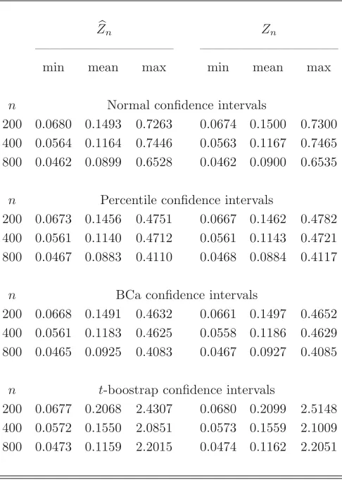
confidence intervals by one-sixth times the standardized third moment of the influence values. In Table 3.2 we report summary statistics concerning the size of the 10,000 confidence intervals. As expected, the confidence intervals based onZn andZn exhibit
[image:10.612.186.429.289.630.2]similar characteristics. We observe from Table 3.1 that all the confidence intervals suffer from some undercoverage. For example, about 97.5% of the studentized bootstrap confidence intervals with 0.99 nominal confidence level contain the true value of the Zenga index. It should be noted that the higher coverage accuracy of the studentized bootstrap confidence intervals (when compared to other ones) comes at the cost of their larger sizes, as seen in Table 3.2. Some of the studentized bootstrap confidence
Table 3.2. Size of the 95% asymptotic confidence intervals from the Pareto parent distribution withx0 = 1 andθ= 2.06 (ZF = 0.6).
Zn Zn
——————————– ——————————–
min mean max min mean max
n Normal confidence intervals
200 0.0680 0.1493 0.7263 0.0674 0.1500 0.7300
400 0.0564 0.1164 0.7446 0.0563 0.1167 0.7465
800 0.0462 0.0899 0.6528 0.0462 0.0900 0.6535
n Percentile confidence intervals
200 0.0673 0.1456 0.4751 0.0667 0.1462 0.4782
400 0.0561 0.1140 0.4712 0.0561 0.1143 0.4721
800 0.0467 0.0883 0.4110 0.0468 0.0884 0.4117
n BCa confidence intervals
200 0.0668 0.1491 0.4632 0.0661 0.1497 0.4652
400 0.0561 0.1183 0.4625 0.0558 0.1186 0.4629
800 0.0465 0.0925 0.4083 0.0467 0.0927 0.4085
n t-boostrap confidence intervals
200 0.0677 0.2068 2.4307 0.0680 0.2099 2.5148
400 0.0572 0.1550 2.0851 0.0573 0.1559 2.1009
800 0.0473 0.1159 2.2015 0.0474 0.1162 2.2051
intervals extend beyond the range of the Zenga index, but this can easily be fixed by taking the minimum between the currently recorded upper bounds and 1, which is the upper bound of the Zenga index ZF for every cdf F. We note that for the BCa
be increased beyond 9,999 if the nominal confidence level is high. Indeed, for samples of size 800, it turns out that the upper bound of 1,598 (out of 10,000) of the BCa confidence intervals based on Zn and with 0.99 nominal confidence level is given by
the largest order statistics of the bootstrap distribution. For the confidence intervals based on Zn, the corresponding figure is 1,641.
4. An analysis of Italian income data
Here we use the Zenga index to analyze data from the Bank of Italy’s Survey on Household Income and Wealth. The sample of the 2006 wave of this survey contain 7,768 households, with 3,957 of them being panel households. For detailed informa-tion on the survey, we refer to the Bank of Italy (2006) publicainforma-tion. In order to treat data correctly in the case of different household sizes, we work with equivalent incomes, which we have obtained by dividing the total household income by an equivalence coef-ficient, which is the sum of weights assigned to each household member. Following the modified OECD (Organization for Economic Cooperation and Developement) equiva-lence scale, we give weight 1 to the household head, 0.5 to the other adult members of the household, and 0.3 to the members under 14 years of age.
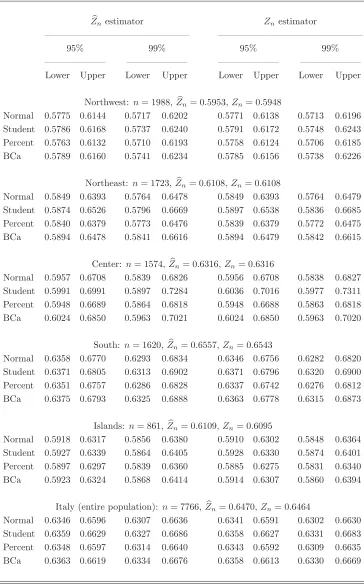
In Table 4.1 we report the values of Zn andZn according to the geographic area of
households, and we also report confidence intervals forZF based on the two estimators.
We note that two households in the sample had negative incomes in 2006 and so we have not included them in our computations. Consequently, the point estimates of ZF are based on 7,766 equivalent incomes with values Zn = 0.6470 and Zn =
0.6464. As pointed out by Maasoumi (1994), however, good care is needed when comparing point estimates of inequality measures. Indeed, direct comparison of the point estimates corresponding to the five geographical areas of Italy would lead us to the erroneous conclusion that the inequality is higher in the central and southern areas when compared to the northern area and the islands. But as we glean from pairwise comparisons of the confidence intervals, only the differences between the estimates corresponding to the northwestern and southern areas and perhaps to the islands and the southern area may be deemed statistically significant.
Moreover, we have used the 3,957 panel households to check whether the Zenga inequality index has changed from the year 2004 to 2006. Table 4.2 reports the values of Zn based on the panel households for these two years, and the 95% confidence
Table 4.1. Confidence intervals for ZF in the 2006 Italian income distribution
Zn estimator Znestimator
———————————————– ———————————————–
95% 99% 95% 99%
——————– ——————– ——————– ——————–
Lower Upper Lower Upper Lower Upper Lower Upper
Northwest: n= 1988,Zn= 0.5953,Zn= 0.5948
Normal 0.5775 0.6144 0.5717 0.6202 0.5771 0.6138 0.5713 0.6196
Student 0.5786 0.6168 0.5737 0.6240 0.5791 0.6172 0.5748 0.6243
Percent 0.5763 0.6132 0.5710 0.6193 0.5758 0.6124 0.5706 0.6185
BCa 0.5789 0.6160 0.5741 0.6234 0.5785 0.6156 0.5738 0.6226
Northeast: n= 1723,Zn= 0.6108,Zn= 0.6108
Normal 0.5849 0.6393 0.5764 0.6478 0.5849 0.6393 0.5764 0.6479
Student 0.5874 0.6526 0.5796 0.6669 0.5897 0.6538 0.5836 0.6685
Percent 0.5840 0.6379 0.5773 0.6476 0.5839 0.6379 0.5772 0.6475
BCa 0.5894 0.6478 0.5841 0.6616 0.5894 0.6479 0.5842 0.6615
Center: n= 1574,Zn= 0.6316,Zn= 0.6316
Normal 0.5957 0.6708 0.5839 0.6826 0.5956 0.6708 0.5838 0.6827
Student 0.5991 0.6991 0.5897 0.7284 0.6036 0.7016 0.5977 0.7311
Percent 0.5948 0.6689 0.5864 0.6818 0.5948 0.6688 0.5863 0.6818
BCa 0.6024 0.6850 0.5963 0.7021 0.6024 0.6850 0.5963 0.7020
South: n= 1620,Zn= 0.6557,Zn= 0.6543
Normal 0.6358 0.6770 0.6293 0.6834 0.6346 0.6756 0.6282 0.6820
Student 0.6371 0.6805 0.6313 0.6902 0.6371 0.6796 0.6320 0.6900
Percent 0.6351 0.6757 0.6286 0.6828 0.6337 0.6742 0.6276 0.6812
BCa 0.6375 0.6793 0.6325 0.6888 0.6363 0.6778 0.6315 0.6873
Islands: n= 861,Zn= 0.6109,Zn= 0.6095
Normal 0.5918 0.6317 0.5856 0.6380 0.5910 0.6302 0.5848 0.6364
Student 0.5927 0.6339 0.5864 0.6405 0.5928 0.6330 0.5874 0.6401
Percent 0.5897 0.6297 0.5839 0.6360 0.5885 0.6275 0.5831 0.6340
BCa 0.5923 0.6324 0.5868 0.6414 0.5914 0.6307 0.5860 0.6394
Italy (entire population): n= 7766,Zn= 0.6470,Zn= 0.6464
Normal 0.6346 0.6596 0.6307 0.6636 0.6341 0.6591 0.6302 0.6630
Student 0.6359 0.6629 0.6327 0.6686 0.6358 0.6627 0.6331 0.6683
Percent 0.6348 0.6597 0.6314 0.6640 0.6343 0.6592 0.6309 0.6635
Table 4.2. 95% confidence intervals for the difference of the Zenga indices between 2006 and 2004 in the Italian income distribution
Northwest (926 pairs) Northest (841 pairs) Center (831 pairs)
Zn(2006) 0.5797 Z
(2006)
n 0.6199 Z
(2006)
n 0.5921
Zn(2004) 0.5955 Z
(2004)
n 0.6474 Z
(2004)
n 0.5766
Difference -0.0158 Difference -0.0275 Difference 0.0155
Lower Upper Lower Upper Lower Upper
Normal -0.0426 0.0102 -0.0573 0.0003 -0.0183 0.0514
Student -0.0463 0.0103 -0.0591 0.0017 -0.0156 0.0644
Percent -0.0421 0.0108 -0.0537 0.0040 -0.0183 0.0505
BCa -0.0440 0.0087 -0.0551 0.0022 -0.0130 0.0593
South (843 pairs) Islands (512 pairs) Italy (3953 pairs)
Zn(2006) 0.6200 Z
(2006)
n 0.6179 Z
(2006)
n 0.6362
Zn(2004) 0.6325 Z
(2004)
n 0.6239 Z
(2004)
n 0.6485
Difference -0.0125 Difference -0.0060 Difference -0.0123
Lower Upper Lower Upper Lower Upper
Normal -0.0372 0.0129 -0.0333 0.0213 -0.0259 0.0007
Student -0.0365 0.0166 -0.0351 0.0222 -0.0264 0.0013
Percent -0.0372 0.0131 -0.0333 0.0214 -0.0253 0.0016
BCa -0.0351 0.0162 -0.0331 0.0216 -0.0255 0.0013
four households with at least one negative income in the paired sample, we are left with a total of 3,953 observations. As before, we see that even though we deal with large sample sizes, the point estimates alone are not reliable. Indeed, for Italy as the whole and for all geographic areas except the center, the point estimates suggest that the Zenga index decreased from the year 2004 to 2006. However, the 95% confidence intervals in Table 4.2 suggest that this change is not significant.
5. An alternative look at the Zenga index
In various contexts we have notions of rich and poor, large and small, risky and secure. They divide the underlying population into two parts, which we can view as sub-populations. The quantile
F−1(p) = inf
{x: F(x)≥p}
mean value of the former sub-population gives rise to the upper conditional expectation
E[X|X > F−1(p)], which is known in the actuarial risk theory as the conditional tail
expectation. Calculating the mean value of the latter sub-population gives rise to the lower conditional expectation E[X|X ≤ F−1(p)], which is known in the econometric
literature as the absolute Bonferroni curve, as a function ofp. The ratio
RF(p) =
E[X|X ≤F−1(p)]
E[X|X > F−1(p)]
of the lower and upper conditional expectations takes on values in the interval [0,1], as we show in the next lemma.
Lemma 5.1. For every p∈(0,1), we have that RF(p)∈[0,1].
Proof. We rewrite the ratio RF(p) as follows:
RF(p) =
E[Xw1(X)]
E[w1(X)]
E[Xw2(X)] E[w2(X)]
, (5.1)
where w1(x) = −1{x ≤ F−1(p)} and w2(x) = 1{x > F−1(p)}. Both functions w1(x)
and w2(x) are non-decreasing, and so by Lemma 3 on p. 1140 of Lehmann (1966) we
have that E[Xw1(X)]≥E[X]E[w1(X)] andE[Xw2(X)]≥E[X]E[w2(X)]. Hence, the
ratio E[Xw1(X)]/E[w1(X)] is not larger than E[X] (note that E[w1(X)] is negative)
and the ratioE[Xw2(X)]/E[w2(X)] is not smaller thanE[X]. Consequently, the
right-hand side of equation (5.1) does not exceed 1. This proves Lemma 5.1.
WhenX is a constant, which can be interpreted as ‘egalitarian’ case, thenRF(p) is
equal to 1. The ratio RF(p) is equal to 0 for all p ∈(0,1) when the lower conditional
expectation is equal to 0 for allp∈(0,1) which means extreme inequality in the sense that, loosely speaking, there is only one individual who possesses the entire wealth. Our wish to associate the egalitarian case with 0 and the extreme inequality with 1 leads to curve 1−RF(p), which coincides with the Zenga curve (see equation (1.2))
when the cdf F is continuous. The area
1−
1
0
E[X|X≤F−1(p)]
E[X|X > F−1(p)]dp
=ZF whenF is continuous
(5.2)
beneath the curve 1−RF(p) is always in the interval [0,1] as follows from Lemma 5.1.
to the absolute Bonferroni curve p−1AL
F(p) and the dual absolute Bonferroni curve
(1−p)−1(μ
F −ALF(p)), respectively, where
ALF(p) =
p
0
F−1(t)dt
is the absolute Lorenz curve. This leads us to the expression of the Zenga index ZF
given by equation (1.1), which we rewrite in terms of the just introduced absolute
Lorenz curve as follows:
ZF = 1−
1
0
1
p−1
ALF(p)
μF −ALF(p)
dp. (5.3)
We shall extensively use expression (5.3) in the proofs below.
6. A closer look at the two Zenga estimators
Since samples are ‘discrete populations’, equations (5.2) and (5.3) lead to slightly different empirical estimators ofZF. If we choose equation (1.1), then we arrive at the
estimatorZn, as seen from the proof of the following theorem.
Theorem 6.1. The empirical Zenga index Zn is an empirical estimator of ZF.
Proof. Let U be a uniform on [0,1] random variable independent of X. The cdf of
F−1(U) is F. Hence, we have the following equations:
ZF = 1−EU
EX[X|X ≤F−1(U)]
EX[X|X > F−1(U)]
= 1−
(0,∞)
1−F(x)
F(x)
E[X1{X ≤x}]
E[X1{X > x}]dF(x)
= 1−
(0,∞)
1−F(x)
F(x)
(0,x]ydF(y)
(x,∞)ydF(y)
dF(x). (6.1)
Replacing every F on the right-hand side of equation (6.1) by Fn, we obtain
1− 1n
n−1
i=1
1−Fn(Xi:n)
Fn(Xi:n)
n
k=1Xk:n1{Xk:n ≤Xi:n}
n
k=1Xk:n1{Xk:n > Xi:n}
,
which simplifies to
1− 1
n
n−1
i=1
1−i/n i/n
i
k=1Xk:n
n
k=i+1Xk:n
.
If we choose equation (5.3) as the starting point for constructing an estimator for
ZF, then we replace the quantile F−1(p) by its empirical counterpart
F−1
n (p) = inf{x: Fn(x)≥p}.
=Xi:n when p∈
(i−1)/n, i/n
in the definition ofALF(p), which gives us the empirical absolute Lorenz curveALn(p),
and then we replace each ALF(p) on the right-hand side of equation (5.3) by the just
constructed ALn(p). (Note that μF = ALF(1) ≈ ALn(1) = ¯X.) This gives us the
empirical Zenga index Zn as seen from the proof of the following theorem.
Theorem 6.2. The empirical Zenga index Zn is an estimator of ZF.
Proof. By construction, the estimator Zn is given by the equation:
Zn= 1−
1
0
1
p −1
ALn(p)
X−ALn(p)
dp. (6.2)
Hence, the proof of the lemma reduces to verifying that the right-hand sides of equations
(2.2) and (6.2) coincide. For this, we split the integral in equation (6.2) into the sum of
integrals over the intervals ((i−1), i/n) fori= 1, . . . , n. For everyp∈((i−1)/n, i/n), we haveALn(p) =Ci,n+pXi:n, where
Ci,n=
1
n
i−1
k=1
Xk:n−
i−1
n Xi:n. (6.3)
Hence, equation (6.2) can be rewritten asZn =ni=1ζi,n, where
ζi,n=
1
n − i/n
(i−1)/n
1
p −1
Λi,n+p
Ψi,n−p
dp
with
Λi,n=
Ci,n
Xi:n
and Ψi,n=
X−Ci,n
Xi:n
. (6.4)
Consider the casei= 1. We haveC1,n= 0 and thus Λ1,n= 0, which implies
ζ1,n=
X X1:n −
1
log
1 +nX1:n k=2Xk:n
.
Next, consider the case i = n. We have Cn,n = X−Xn:n and thus Ψn,n = 1, which
implies
ζn,n=
1− X
Xn:n
log
n n−1
When 2 ≤ i ≤ n−1, then the integrand in the definition of ζi,n does not have any
singularity, since Ψi,n> i/ndue to
n
k=i+1Xk:n >0 almost surely. Hence, after simple
integration we have that, for i= 2, . . . , n−1,
ζi,n=
(i−1)Xi:n−i
−1
k=1Xk:n
n
k=i+1Xk:n+iXi:n
log
i i−1
+
X Xi:n −
1 + (i−1)Xi:n−
i−1
k=1Xk:n
n
k=i+1Xk:n+iXi:n
log
1 +nXi:n k=i+1Xk:n
.
With the above formulas forζi,n we easily check that the sum
n
i=1ζi,n is equal to the
right-hand side of equation (2.2). This completes the proof of Theorem 6.2.
7. A closer look at variances
Following the formulation of Theorem 2.1 we claimed that the asymptotic distribu-tion of √n(Zn−ZF) is centered normal with the finite variance σF2 =E[h2(X)]. The
following theorem provides a proof of this claim.
Theorem 7.1. When E[X2+α]<
∞for some α >0, then n−1/2n
i=1h(Xi) converges
in distribution to the centered normal random variable
Γ =
∞
0 B
(F(x))wF(F(x))dx,
where B is the Brownian bridge on the interval [0,1]. The variance of Γ is finite and equal to σ2
F.
Proof. Note that n−1/2n
i=1h(Xi) can be written as
∞
0 en(F(x))wF(F(x))dx, where
en(p) =√n(En(p)−p) is the empirical process based on the uniform on [0,1] random
variablesUi=F(Xi), i= 1, . . . , n. We shall next show that
∞
0
en(F(x))wF(F(x))dx→d
∞
0 B
(F(x))wF(F(x))dx. (7.1)
The proof is based on the well known fact that, for everyε >0,
en(p)
p1/2−ε(1−p)1/2−ε, 0≤p≤1
⇒
B(p)
p1/2−ε(1−p)1/2−ε, 0≤p≤1
.
Hence, in order to prove statement (7.1), we only need to check that the integral
∞
0
F(x)1/2−ε(1
−F(x))1/2−εw
is finite. For this, by considering the two cases p ≤ 1/2 and p > 1/2 separately, we easily show that |wF(p)| ≤ c+clog(1/p) +clog(1/(1−p)). Hence, for every ε > 0,
there exists a constantc <∞ such that, for allp∈(0,1),
|wF(p)| ≤
c
pε(1−p)ε. (7.3)
Bound (7.3) implies that integral (7.2) is finite provided that 0∞(1−F(x))1/2−2εdx
is finite, which is true since the moment E[X2+α] is finite for some α > 0 and the
parameter ε > 0 can be chosen as small as desired. Hence, n−1/2n
i=1h(Xi) →d Γ
with Γ denoting the integral on the right-hand side of statement (7.1). The random
variable Γ is normal because the Brownian bridge is a Gaussian process. Furthermore,
Γ has mean zero becauseB(p) has mean zero for everyp∈[0,1]. The variance of Γ is equal to σ2
F becauseE[B(p)B(q)] = min{p, q} −pq for all p, q ∈ [0,1]. We are left to
show that E[Γ2]<∞. For this, we write the bound:
E[Γ2] =
∞
0
∞
0
E[B(F(x))B(F(y))]wF(F(x))wF(F(y))dxdy
≤
∞
0
E[B2(F(x))]w
F(F(x))dx
2
. (7.4)
Since E[B2(F(x))] = F(x)(1−F(x)), the finiteness of the integral on the right-hand
side of bound (7.4) follows from the earlier proved statement that integral (7.2) is finite.
Hence, E[Γ2]<∞, which concludes the proof of Theorem 7.1.
Theorem 7.2. The empirical varianceS2
X,n is an estimator of σF2.
Proof. We construct an empirical estimator for σ2
F by replacing every F(x) on the
right-hand side of equation (2.4) by the empiricalFn(x). In particular, we replace the
function wF(t) by its empirical version
wX,n(t) =−
t
0
1
p −1
ALn(p)
(X−ALn(p))2
dp+
1
t
1
p −1
1
X−ALn(p)
dp.
We denote the just defined estimator of σ2
F by SX,n2 , and the rest of the proof consists
of showing that the estimator S2
X,n coincides with the one defined by equation (2.6).
Note that min{Fn(x), Fn(y)} −Fn(x)Fn(y) = 0 when x∈[0, X1:n)∪[Xn:n,∞) and/or
y∈[0, X1:n)∪[Xn:n,∞). Hence, the just defined SX,n2 is equal to
Xn:n
X1:n
Xn:n
X1:n
min{Fn(x), Fn(y)} −Fn(x)Fn(y)
SinceFn(x) =k/n whenx∈[Xk:n, Xk+1:n), we therefore have that
SX,n2 = n−1
k=1
n−1
l=1
min{k, l}
n − k n l n
×wX,n
k n wX,n l n
(Xk+1:n−Xk:n)(Xl+1:n−Xl:n).
Furthermore, wX,n k n =− k/n 0 1
p −1
ALn(p)
(X−ALn(p))2
dp+
1
k/n
1
p −1
1
X−ALn(p)
dp
=−
k
i=1
IX,n(i) + n
i=k+1
JX,n(i), (7.5)
where, using notations (6.3) and (6.4), the summands on the right-hand side of equation
(7.5) are:
IX,n(i) =
1
Xi:n
i/n
(i−1)/n
1
p −1
Λi,n+p
(Ψi,n−p)2
dp
for alli= 1, . . . , n−1, and
JX,n(i) =
1
Xi:n
i/n
(i−1)/n
1
p −1
1 Ψi,n−p
dp
for alli= 2, . . . , n. Wheni= 1, then Λi,n = 0, and we easily check the expression for
IX,n(1) given by equation (2.7). When 2≤i≤n−1, then
IX,n(i) =
Λi,n
Xi:nΨ2i,n
log
i i−1
− (Λi,n+ Ψi,n)(Ψi,n−1)
nXi:nΨi,n
Ψi,n−(i−1)/n
Ψi,n−i/n
+ 1
Xi:n
1 + Λi,n Ψ2
i,n
log
Ψi,n−(i−1)/n
Ψi,n−i/n
,
and, after some algebra, we arrive at the right-hand side of equation (2.8). When
2≤i≤n−1, then we have
JX,n(i) =
1
Xi:nΨi,n
log
i i−1
− X1
i:n
1−Ψ1
i,n
log
Ψi,n−(i−1)/n
Ψi,n−i/n
,
which, after some algebra, becomes equation (2.9). When i = n, then Ψi,n = 1, and
we thus easily see thatJX,n(i) is given by equation (2.10). This completes the proof of
Theorem 7.2.
Proof. We proceed similarly to the proof of Theorem 7.2. We estimate the integrand
P[X≤x, Y ≤y]−F(x)H(y) using
1
n
n
i=1
1{Xi ≤x, Yi≤y} −
1
n
n
i=1
1{Xi≤x}
1
n
n
i=1
1{Yi ≤y}. (7.6)
After some rearrangement of terms, estimator (7.6) becomes
1
n
n
i=1
1{Xi:n≤x, Y(i,n)≤y} −
1
n
n
i=1
1{Xi:n≤x}
1
n
n
i=1
1{Yi:n ≤y}. (7.7)
Whenx∈[Xk:n, Xk+1:n) andy∈[Yl:n, Yl+1:n), then estimator (7.7) isn−1ki=11{Y(i,n)≤
Yl:n} −(k/n)(l/n), which leads us to the estimatorSX,Y,nand thus completes the proof
of Theorem 7.3.
8. Proof of Theorem 2.1
Throughout the proof we conveniently use the notationAL∗
F(p) for the dual absolute
Lorenz curvep1F−1(t)dt, which is equal toμ
F−ALF(p). Likewise, we use the notation
AL∗
n(p) for the empirical dual absolute Lorenz curve. Hence,
√
n(Zn−ZF) =−√n
1
0
1
p −1
ALn(p)
AL∗
n(p)
−ALALF∗(p)
F(p)
dp.
Simple algebra gives the representation
√
n(Zn−ZF) =−√n
1
0
1
p −1
ALn(p)−ALF(p)
AL∗
F(p)
dp
+√n 1
0
1
p −1
ALF(p)
AL∗2
F(p)
(AL∗
n(p)−AL
∗
F(p))dp
−rn,1+rn,2, (8.1)
where the two remainder terms are:
rn,1=√n
1
0
1
p−1
(ALn(p)−ALF(p))
1
AL∗
n(p) −
1
AL∗
F(p)
dp
and
rn,2 =√n
1
0
1
p −1
ALF(p)
AL∗
F(p)
(AL∗
n(p)−AL
∗
F(p))
1
AL∗
n(p)
−AL1∗
F(p)
dp.
We shall later show (Lemmas 9.1 and 9.2 below) that the remainder termsrn,1 andrn,2
are of the order oP(1). Hence, we proceed with an analysis of the first two terms on the right-hand side of equation (8.1), for which we use the (general) Vervaat process
Vn(p) =
p
0
(F−1
n (t)−F
−1(t))dt+
F−1(p)
0
and its dual version
V∗
n(p) =
1
p
(F−1
n (t)−F
−1(t))dt+
∞
F−1(p)
(Fn(x)−F(x))dx. (8.3)
For mathematical and historical details on the Vervaat process, see Zitikis (1998), Greselin et al. (2009), and references therein. Since 01(F−1
n (t)−F
−1(t))dt=X−μ
F
and0∞(Fn(x)−F(x))dx=−(X−μF), adding the right-hand sides of equations (8.2)
and (8.3) gives the equationV∗
n(p) = −Vn(p). Hence, whatever upper bound we have
for |Vn(p)|, the same bound also holds for |Vn∗(p)|. In fact, the absolute value can be
dropped from |Vn(p)| since Vn(p) is non-negative. Among other facts that we know
aboutVn(p) is that it does not exceed (p−Fn(F−1(p)))(Fn−1(p)−F
−1(p)). Hence, with
en(p) =√n(Fn(F−1(p))−p), which is the uniform on [0,1] empirical process, we have
that
√
n Vn(p)≤
en(p)
F−1
n (p)−F
−1(p). (8.4)
Bound (8.4) implies the following asymptotic representation for the first term on the right-hand side of equation (8.1):
−√n 1
0
1
p −1
ALn(p)−ALF(p)
AL∗
F(p)
dp
=√n 1
0
1
p −1
1
AL∗
F(p)
F−1(p)
0
(Fn(x)−F(x))dx
dp+OP(rn,3), (8.5)
where
rn,3=
1
0
1
p −1
1
AL∗
F(p)
en(p)
F−1
n (p)−F
−1(p)dp.
We shall later show (Lemma 9.3 below) that rn,3 = oP(1). Furthermore, we have the following asymptotic representation for the second term on the right-hand side of equation (8.1): √ n 1 0 1
p −1
ALF(p)
AL∗2
F(p)
(AL∗
n(p)−AL
∗
F(p))dp
=−√n 1
0
1
p −1
ALF(p)
AL∗2
F(p)
∞
F−1(p)
(Fn(x)−F(x))dx
dp+OP(rn,4), (8.6)
where
rn,4 =
1
0
1
p−1
ALF(p)
AL∗2
F(p)
en(p)
F−1
n (p)−F
−1
We shall later show (Lemma 9.4 below) thatrn,4 =oP(1). Hence, equations (8.1), (8.5)
and (8.6) together with the statements rn,1, . . . , rn,4 =oP(1) imply that
√
n(Zn−ZF) =√n
1
0
1
p −1
1
AL∗
F(p)
F−1(p)
0
(Fn(x)−F(x))dx
dp
−√n 1
0
1
p−1
ALF(p)
AL∗2
F(p)
∞
F−1(p)
(Fn(x)−F(x))dx
dp+oP(1)
=√1n
n
i=1
h(Xi) +oP(1),
which completes the proof of Theorem 2.1.
9. Negligibility of remainder terms
The following four lemmas establish the earlier noted statements that the remainder terms rn,1, . . . , rn,4 are of the orderoP(1). In the proofs of the lemmas we shall use a
parameter δ ∈ (0,1/2], possibly different from line to line but never depending on n. Furthermore, we shall frequently use the fact that
E[Xq]<∞ =⇒
1
0
F−1
n (t)−F
−1(t)qdt=o
P(1). (9.1)
Another technical result that we shall frequently use is the fact that, for any ε >0 as small as desired,
sup
x∈R
√n
|Fn(x)−F(x)|
F(x)1/2−ε(1−F(x))1/2−ε =OP(1) (9.2)
whenn→ ∞.
Lemma 9.1. Under the conditions of Theorem 2.1, we have that rn,1 =oP(1).
Proof. We split the remainder term rn,1 = √n
1
0 . . . dp into the sum of r
∗
n,1(δ) =
√n1−δ
0 . . . dp andr
∗∗
n,1(δ) =
√n1
1−δ. . . dp. The lemma follows if: (1) For everyδ > 0, the statementr∗
n,1(δ) =oP(1) holds when n→ ∞.
(2) r∗∗
n,1(δ) =h(δ)OP(1) for a deterministic h(δ)↓0 when δ ↓0, whereOP(1) does not depend on δ.
To prove part (1), we first note that when 0< p <1−δ, thenAL∗
F(p)≥
1 1−δF
−1(t)dt,
which is positive, andAL∗
n(p)≥
1 1−δF
−1(t)dt+oP(1) due to statement (9.1) withq= 1.
Hence, we are left to show that, when n→ ∞,
√
n 1−δ
0
1
p|ALn(p)−ALF(p)| |AL ∗
n(p)−AL
∗
SinceAL∗
n(p)−AL
∗
F(p) = (X−μF)−(ALn(p)−ALF(p)), statement (9.3) follows if
√
n|X−μF|
1−δ
0
1
p|ALn(p)−ALF(p)|dp=oP(1) (9.4)
and
√
n 1−δ
0
1
p|ALn(p)−ALF(p)|
2dp=o
P(1). (9.5)
We have√n|X−μF|=OP(1) and|ALn(p)−ALF(p)| ≤√p(
1 0 |F
−1
n (p)−F
−1(p)|2dp)1/2.
Since 01|F−1
n (p)−F
−1(p)
|2dp = oP(1) and 1−δ
0 p
−1√p dp <
∞, we have statement (9.4). To prove statement (9.5), we use bound (8.4) and reduce the proof to showing
that
1
√
n 1−δ
0 1 p
F−1(p)
0
√
n(Fn(x)−F(x))dx
2
dp=oP(1) (9.6)
and
1
√
n 1−δ
0
1
p en(p)
2
F−1
n (p)−F
−1(p)2dp=oP(1). (9.7)
To prove statement (9.6), we use statement (9.2) and observe that
1−δ
0
1
p
F−1(p)
0
F(x)1/2−ε dx
2
dp≤c(F, δ)
1−δ
0
1
pp
1−2ε
dp <∞. (9.8)
To prove statement (9.7), we use the uniform on [0,1] version of statement (9.2) and
H¨older’s inequality, and in this way reduce the proof to showing that
1
√
n
1−δ
0
1
p2εadp
1/a 1−δ
0
F−1
n (p)−F
−1(p)2bdp
1/b
=oP(1) (9.9)
for some a, b > 1 such that a−1+b−1 = 1. We choose aand b as follows. First, since E[X2+α] < ∞, we set b = (2 +α)/2. Next, we choose ε > 0 on the left-hand side
of statement (9.9) so that 2εa < 1, which holds when ε < α/(4 + 2α) in view of the
equationa−1+b−1 = 1. Hence, statement (9.9) holds and thus statement (9.7) follows.
This completes the proof of part (1).
To establish part (2), we first estimate|r∗∗
n,1(δ)|from above using the boundsAL
∗
F(p) ≥
(1−p)F−1(1/2) and AL∗
n(p) ≥ (1−p)F
−1
n (1/2), which hold since δ ≤ 1/2. Hence,
we have reduced our task to showing that√n11−δ|ALn(p)−ALF(p)|dp=h(δ)OP(1).
Using the Vervaat process, we reduce the latter statement to showing that the integrals
1
1−δ
F−1(p)
0
√
n|Fn(x)−F(x)|dx
dp (9.10)
and
1
1−δ
en(p)
F−1
n (p)−F
are of the order h(δ)OP(1) with possibly different h(δ) ↓ 0 in each case. In view of statement (9.2), we have the desired statement for integral (9.10) if the quantity
1
1−δ
F−1(p)
0
(1−F(x))1/2−εdx
dp (9.12)
converges to 0 whenδ ↓0, in which case we set the quantity to be ourh(δ). The inner integral of (9.12) does not exceed0∞(1−F(x))1/2−εdx, which is finite for all sufficiently
smallε >0 sinceE[X2+α]<
∞for someα >0. This completes the proof that quantity (9.10) is of the orderh(δ)OP(1). To show that quantity (9.11) is of the same order, we
use the uniform on [0,1] version of statement (9.2) and reduce the task to showing that
1 1−δ|F
−1
n (p)−F
−1(p)|dpis of the desired order. By the Cauchy-Bunyakowski-Schwarz
inequality, we have
1
1−δ|
F−1
n (p)−F
−1(p)
|dp≤√δ
1 0 |
F−1
n (p)−F
−1(p)
|2dp
1/2
.
SinceE[X2]<
∞, we have01|F−1
n (p)−F
−1(p)
|2dp=o
P(1), and so settingh(δ) =
√
δ
establishes the desired asymptotic result for integral (9.11). This also completes the
proof of part (2) and also of Lemma 9.1.
Lemma 9.2. Under the conditions of Theorem 2.1, we have that rn,2 =oP(1).
Proof. Like in the proof of Lemma 9.1, we split the remainder termrn,2 =√n
1 0 . . . dp
into the sum of r∗
n,2(δ) =
√
n01−δ. . . dp and r∗∗
n,2(δ) =
√
n11−δ. . . dp. To prove the
lemma, we need to show that:
(1) For everyδ > 0, the statementr∗
n,2(δ) =oP(1) holds when n→ ∞.
(2) r∗∗
n,2(δ) =h(δ)OP(1) for a deterministic h(δ)↓0 when δ ↓0, whereOP(1) does
not depend on δ.
To prove part (1), we first estimate|r∗
n,2(δ)|from above using the boundsp
−1AL
F(p)≤
F−1(1−δ) < ∞, AL∗
F(p) ≥
1 1−δF
−1(t)dt > 0, and AL∗
n(p) ≥
1 1−δF
−1(t)dt+o
P(1). This reduces our task to showing that, for everyδ > 0,
√
n 1−δ
0 |
AL∗
n(p)−AL
∗
F(p)|2dp=oP(1). (9.13) SinceAL∗
n(p)−AL
∗
F(p) = (X−μF)−(ALn(p)−ALF(p)) and√n(X−μF)2=oP(1),
statement (9.13) follows from
√
n 1−δ
0 |
which is an elementary consequence of statement (9.5). This establishes part (1).
To prove part (2), we first estimate|r∗∗
n,2(δ)|from above using the boundsAL
∗
F(p)≥
(1−p)F−1(1/2) and AL∗
n(p) ≥ (1−p)F
−1
n (1/2), and in this way reduce the task to
showing that
√
n 1
1−δ
1 1−p|AL
∗
n(p)−AL
∗
F(p)|dp=h(δ)OP(1). (9.14)
Using the Vervaat process, the proof of statement (9.14) follows if
1
1−δ
1 1−p
∞
F−1(p)
√
n|Fn(x)−F(x)|dx
dp=h(δ)OP(1) (9.15)
and
1
1−δ
1 1−p
en(p)
F−1
n (p)−F
−1(p)dp=h(δ)O
P(1) (9.16)
with possibly different h(δ) ↓ 0 in each case. Using statement (9.2), we have that statement (9.15) holds withh(δ) set as the integral
1
1−δ
1 1−p
∞
F−1(p)
(1−F(x))1/2−εdx
dp, (9.17)
which converges to 0 when δ↓ 0 as the following argument shows. First, we write the integrand as the product of (1−F(x))ε and (1−F(x))1/2−2ε. Then we estimate the
first factor by (1−p)ε. The integral ∞
0 (1−F(x))
1/2−2εdx is finite for all sufficiently
smallε >0 sinceE[X2+α]<∞for someα >0. Since1
1−δ(1−p)
−1+εdp↓0 whenδ ↓0,
integral (9.17) converges to 0 when δ↓0. The proof of statement (9.15) is finished. We are left to prove statement (9.16). Using the uniform on [0,1] version of statement
(9.2), we reduce the task to showing that
1
1−δ
1 (1−p)1/2+ε
F−1
n (p)−F
−1(p)dp=h(δ)O
P(1). (9.18)
(In fact, we shall see below that OP(1) can be replaced by oP(1).) Using H¨older’s
inequality, we have that the right-hand side of equation (9.18) does not exceed
1 1−δ
1
(1−p)(1/2+ε)adp
1/a 1
1−δ
F−1
n (p)−F
−1(p)bdp
1/b
(9.19)
for somea, b >1 such thata−1+b−1= 1, which we choose as follows. SinceE[X2+α]<
∞, we set b = 2 +α, and so the right-most integral of (9.19) is of the order oP(1). Furthermore, a = (2 +α)/(1 +α) < 2, which can be made arbitrarily close to 2 by
choosing sufficiently smallα >0. Choosingε >0 so small that (1/2 +ε)a <1, we have
we set the integral to be our function h(δ). This establishes statement (9.16) and
completes the proof of Lemma 9.2.
Lemma 9.3. Under the conditions of Theorem 2.1, we have that rn,3 =oP(1).
Proof. We split the remainder term rn,3 =
1
0 . . . dp into the sum of r
∗
n,3 =
1/2 0 . . . dp
andr∗∗
n,3=
1
1/2. . . dp. The lemma follows if the two summands are of the order oP(1).
To prove r∗
n,3 = oP(1), we use the bound AL∗F(p) ≥
1 1/2F
−1(p)dpand the uniform
on [0,1] version of statement (9.2), and in this way reduce our task to showing that
1/2
0
1
p1/2+ε
F−1
n (p)−F
−1(p)dp=oP(1).
This statement can be established following the proof of statement (9.18), with minor
modifications.
To prove r∗∗
n,3 = oP(1), we use the bound AL
∗
F(p) ≥ (1−p)F
−1(1/2), the fact that
supt|en(t)|=OP(1), and statement (9.1) withq= 1. The desired result forr∗∗n,3follows,
which finishes the proof of Lemma 9.3.
Lemma 9.4. Under the conditions of Theorem 2.1, we have that rn,4 =oP(1).
Proof. We split rn,4=
1
0 . . . dp into the sum ofr
∗
n,4 =
1/2
0 . . . dp andr
∗∗
n,4=
1
1/2. . . dp,
and then show that the two summands are of the order oP(1).
To prove r∗
n,4 = oP(1), we use the bounds p
−1AL
F(p) ≤ F−1(1/2) < ∞ and
AL∗
F(p) ≥
1 1/2F
−1(p)dp > 0 together with the uniform on [0,1] version of statement
(9.2). This reduces our task to showing that01/2|F−1
n (p)−F
−1(p)
|dp=oP(1), which holds due to statement (9.1) withq = 1.
To prover∗∗
n,4 =oP(1), we use the boundAL
∗
F(p)≥(1−p)F
−1(1/2) and the uniform
on [0,1] version of statement (9.2), and in this way reduce the proof to showing that
1
1/2
1 (1−p)1/2+ε
F−1
n (p)−F
−1(p)dp=o
P(1).
This statement can be established following the proof of statement (9.18). The proof
of Lemma 9.4 is finished.
References
Davison A.C., Hinkley D.V. (1997). Bootstrap Methods and their Application. Cambridge University Press, Cambridge.
Efron B.(1987). Better bootstrap confidence intervals (with discussion). Journal of the American Statistical Association, 82, 171–200.
Gastwirth, J.L.(1971). A general definition of the Lorenz curve. Econometrica, 39, 1037–1039.
Gini C.(1914). Sulla misura della concentrazione e della variabilit´a dei caratteri. In:
Atti del Reale Istituto Veneto di Scienze, Lettere ed Arti. Anno Accademico 1913– 1914, Tomo LXXII parte seconda. Premiate Officine Grafiche C. Ferrari, Venezia, 1201–1248.
Greselin, F. and Pasquazzi, L.(2009). Asymptotic confidence intervals for a new inequality measure. Communications in Statistics: Computation and Simulation, 38(8), 17-42.
Greselin, F., Puri, M.L. and Zitikis, R. (2009). L-functions, processes, and statistics in measuring economic inequality and actuarial risks. Statistics and Its Interface, 2, 227–245.
Karian, Z.A. and Dudewicz, E.J. (2000). Fitting Statistical Distributions: The Generalized Lambda Distribution and Generalized Bootstrap Methods. CRC Press, Boca Raton, FL.
Kleiber, C. and Kotz, S. (2003). Statistical Size Distributions in Economics and Actuarial Sciences. Wiley, New York.
Lehmann, E.L. (1966). Some concepts of dependence. Annals of Mathematical Sta-tistics, 37, 1137–1153.
Maasoumi E. (1994). Empirical analysis of welfare and inequality. In: Handbook of Applied Econometrics, Volume II: Microeconomics. (Eds.: M.H. Pesaran and P. Schmidt). Blackwell, Oxford.
Pietra G. (1915). Delle relazioni fra indici di variabilit´a, note I e II. Atti del Reale Istituto Veneto di Scienze, Lettere ed Arti, 74, 775-804.
Zenga, M.(2007). Inequality curve and inequality index based on the ratios between lower and upper arithmetic means. Statistica & Applicazioni 5, 3–27.