Generation of Narrow Beams using differential Evolution
Algorithm from Circular Arrays
G. S. K. Gayatri Devi
Research Scholar Dept. of Electronics and Communication Engineering AU College of Engineering(A)
Andhra University Visakhapatnam, Andhra
Pradesh India-530 003
G. S. N. Raju
Professor Dept. of Electronics and Communication Engineering AU College of Engineering(A)
Andhra University Visakhapatnam, Andhra
Pradesh India-530 003
P. V. Sridevi
Professor Dept. of Electronics and Communication Engineering AU College of Engineering(A)
Andhra University Visakhapatnam, Andhra
Pradesh India-530 003
ABSTRACT
Concentric circular arrays are increasingly shown more interest in antenna design for generating low sidelobe patterns as they have radial symmetry and an invariant beam in the azimuthal plane. Such patterns are desirable in low EMI applications. In the present work, an attempt is made to generate low sidelobe patterns from concentric circular arrays by optimizing both ring radii and individual element excitations. The array is also subjected to thinning simultaneously. Thinning results in sidelobe reduction while keeping the number of active elements small. For each optimum configuration, the optimal ring radii and the amplitude excitation levels are obtained using Differential Evolution algorithm. Results are presented for 8, 10 concentric rings.
Keywords
Concentric Circular Array Antenna, Array Thinning, Optimization, Sidelobe Reduction, Differential Evolution.
1.
INTRODUCTION
In many applications it becomes necessary to design antennas with directive radiation characteristics. Antenna arrays not only provide high gain but they also increase directivity. Careful design of antenna arrays results in patterns with desired radiation characteristics [1]. Planar arrays have better control than linear arrays over radiation characteristics.
A circular array is a planar array with elements arranged on a circle. A concentric circular array is an array of such circular arrays all sharing same center with different radii [2]. They are given more importance as they have attractive features like compact antenna structure, a beam pattern which remains constant in the azimuthal plane. As there are no edge elements, the directional pattern generated can be easily scanned in the array plane. These are used in various applications like radio direction finding, air and space navigation, mobile, radar and wireless communication applications [3-4].
A Uniform Concentric Circular Array (UCCA) is one where all the elements have an inter element spacing set to half wavelength and are given uniform excitation. Although this array exhibits high directivity, it suffers from high side lobes.
Reduction in side lobe level can be achieved by varying the ring radii, by non-uniformly exciting elements or by placing the elements unequally. A lot of research work was carried out for generating patterns with low side lobe levels. In [5],
array factor for a concentric ring array with constant ring spacing was approximated as a truncated Fourier-Bessel-Series, from which the excitation weights for each ring were obtained to generate chebyshev like pattern. In [6], Goto and Cheng showed that the maximum inter element spacing should be less than
0.4𝜆
for a taylor weighted ring array to avoid appearance of high side lobes. In [7], Biller and Friedman employed steepest descent method to obtain element weights and ring spacing that result in low side lobes as well as control over beamwidth. In [8], Huebner carried out optimization of small concentric ring arrays for low side lobe levels by finding proper ring spacings. Kumar and Branner [9] generated low side lobes from circular arrays by optimizing ring radius. Dessouky et al. [10] showed that low side lobes can be obtained by placing an active element at the centre of concentric array at the cost of small increase in the beamwidth.Array thinning is another technique for generating low side lobe field patterns [11-12]. It results in reduction of cost and weight of the antenna array. Thinning is carried out by removing certain elements from the array without degrading the system performance. The elements which remain ‗ON‘ (active) are given excitation levels necessary for side lobe reduction. Another advantage offered by thinning is that, the beamwidth can be maintained approximately same as for a fully filled array. Aperiodic array synthesis aims at reducing side lobes by strategically placing uniformly weighted elements. Thinning is simpler than aperiodic synthesis as a ‗n‘ element array involves checking of 2n possible combinations only. As ‗n‘ becomes large, traditional methods won‘t work and one has to go for optimization techniques. Many global optimization techniques such as GA [13], PSO [14], BBO [15], Firefly Algorithm [16] etc were successfully applied for thinning of concentric ring arrays. Differential Evolution Algorithm [17] is used in the present work for optimization problem. It is an efficient search algorithm successfully applied for solving many optimization problems [18-20].
side lobes. The simulated results are presented for 8 and 10 rings. All results are simulated using Matlab software.
The paper is organized as follows. Section 2 gives a brief description of DE algorithm. Problem formulation is given in section 3. In section 4, results are presented. Conclusions are discussed in section 5.
2.
DIFFERENTIAL EVOLUTION
ALGORITHM
DE is a simple population based stochastic search algorithm. It was first proposed by Storn and Price [21]. It is another evolutionary algorithm which paved way for solving complex optimization problems. It is a powerful search technique which is successfully applied in many fields like communications, pattern recognition etc. The algorithm offers following advantages:
It can easily handle non-linear, non-differentiable complex cost functions
It has few easy to choose control parameters which influence the convergence of the algorithm
Good convergence speed in finding optimum value
The main steps involved in the algorithm are described as below:
Step 1: Initialization: The algorithm starts with ‗N‘ (at least equal to 4) population vectors. The individuals are called target vectors. The total number of these parameter vectors remains same throughout the algorithm. Let ‗xi,G‘ represent
the ith parameter vector where i=1, 2… N. ‗G‘ is the generation number. The parameter vectors are randomly initialized in step 1.
Step 2: Cost Evaluation: The initial xi,G parameter vectors are
evaluated for their cost using the objective function.
Step 3: Mutation: In this step, new parameter vectors are generated by adding weighted difference between two target vectors to a third target vector, i.e. for a given target vector ‗xi,G‘ , select three target vectors xr1,G , xr2,G , xr3,G such that i,
r1, r2, r3 are distinct to form mutant vectors called ‗donor vectors‘.
𝑉𝑗𝑖 ,𝐺+1= 𝑥𝑟1,𝐺+ 𝐹 𝑥𝑟2,𝐺− 𝑥𝑟3,𝐺
here r1, r2, r3 ∈ {1, 2…, N}
Mutation expands the solution space. The factor ‗F‘ is called mutation factor. Usually it is a real constant chosen in the range 0 to 2.
Step 4: Crossover: It increases the diversity of parameter vectors by including good solutions or vectors from previous generations. It forms the new so called ‗trail vectors (ui,G+1)‘
by mixing elements of target vector ‗xi,G‘, and donor vector
‗vi,G+1‘.
𝑢𝑗𝑖 ,𝐺+1= 𝑣𝑗𝑖 ,𝐺+1 𝑖𝑓 𝑟𝑎𝑛𝑑 ≤ 𝐶𝑅 𝑜𝑟 𝑗 = 𝐼𝑟𝑎𝑛𝑑
= 𝑥𝑗𝑖 ,𝐺+1 𝑖𝑓 𝑟𝑎𝑛𝑑 > 𝐶𝑅 𝑎𝑛𝑑 𝑗 ≠ 𝐼𝑟𝑎𝑛𝑑
Here i=1,2…N; j=1,2…,D. D is the number of parameters in one vector. Irand is a randomly number chosen in the range 1 to
D which ensures that ui,G+1 gets at least one parameter from
vi,G+1. CR is the crossover constant to be taken in the range
(0,1).
Step 5: Selection: It imitates survival-of-the-fittest. It follows greedy scheme and selects vectors for next generation. The process is as follows:
𝑥𝑖,𝐺+1= 𝑢𝑖,𝐺+1 𝑖𝑓 𝑐𝑜𝑠𝑡 𝑢𝑖,𝐺+1 ≤ 𝑐𝑜𝑠𝑡 𝑥𝑖,𝐺
= 𝑥𝑖,𝐺 𝑜𝑡ℎ𝑒𝑟𝑤𝑖𝑠𝑒
That means, the newly generated trial vectors replace parent target vectors if they yield lower cost otherwise the parent target vectors are passed on to next generation.
Step 6: Stopping criteria: Steps 2 to 5 are repeated until some stopping criteria is met. Stopping criteria in general may be fixed number of generations or predetermined cost.
There are different schemes in DE suggested by Storn and Price [21]. In the present work, a DE/rand/1/binary scheme is used.
3.
FORMULATION
The geometry of a ‗m‘ ring concentric circular array with a single element at centre is as shown in figure 1. Assume all elements are isotropic elements. Let rm represent the radius of
mth ring and let the number of elements present in mth ring be Nm where m=1,2,..,M. Let dm be the inter element spacing.
The array factor for the array [22] is given by
𝐸 𝜃 = 1 + 𝐼𝑚𝑛
𝑁𝑚
𝑛=1 𝐴𝑚𝑛 𝑀
𝑚 =1
exp(𝑗𝑘𝑟𝑚sin 𝜃 cos ∅ − ∅𝑚𝑛 )
(1)
where M=number of rings
Nm=Number of elements in ring ‗m‘
Imn=excitation of nth element in mth ring= ‗1‘ for ON
= ‗0‘ for OFF
rm= radius of ring ‗m‘
Amn= Amplitude excitation of nth element in mth ring
∅𝑚𝑛= angular position of nth element of mth ring =2𝜋 𝑚 −1 𝑁
𝑚 (2)
k=2π/λ
θ= elevation angle
∅=azimuthal angle=constant in the present work In ‗u‘ domain
𝐸 𝑢 = 1 + 𝐼𝑚𝑛
𝑁𝑚
𝑛=1 𝑀
𝑚 =1
Amnexp(𝑗𝑘𝑟𝑚𝑢 cos ∅ − ∅𝑚𝑛 )
where u=sinθ
The radius of mth ring is given by rm=mλ/2 (3)
The inter element spacing is assumed to be approximately λ/2 i.e. dm=λ/2
The number of equally spaced elements present in ring ‗m‘ is
given by
𝑁
𝑚=
2𝜋𝑟𝑚𝑑𝑚 (4)
digits present on right of the decimal point were dropped. All the elements have uniform excitation phase of zero degrees.
Present work is divided into two cases. In the first case, an 8 ring concentric array of isotropic sources is considered. The array is excited uniformly and the interelement spacing is set
Figure 1. Concentric Circular array of isotropic antennas
to half wavelength. The number of elements in each ring is calculated using eq. (4). The ring radii are calculated using eq. (3). The resulting far field pattern yields a peak SLL of -17.39dB. Now the array is subjected to thinning. The results show a reduction in peak SLL.
In the second case, both ring radii and amplitude excitations of elements in each ring are optimized. The array is also thinned simultaneously. This resulted in further reduction of side lobes. Results are also presented for 10 rings following the same above mentioned procedure. All the optimum array configurations are acquired by employing a DE algorithm.
The objective function used for calculating the fitness of candidate solutions is as follows:
𝐹𝑖𝑡 = 𝑃𝑆𝐿𝐿𝑜− 𝑆𝐿𝐿𝑑
where 𝑃𝑆𝐿𝐿𝑜= 𝑀𝑎𝑥 20log 𝐸𝐸 𝑢,
𝑀𝑎𝑥 𝑢 u ∈ side lobe region.
SLLd =Desired Sidelobe level
Emax(u)=Main beam peak value
4.
RESULTS
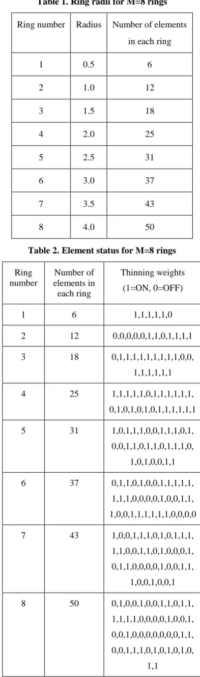
This section presents a brief description of results obtained for concentric circular arrays. An eight ring concentric array of isotropic sources with central element feeding is considered. An interelement spacing of half wavelength is maintained throughout for all optimum array configurations. The ring radii and number of elements in each ring are presented in Table 1. A DE algorithm is used for array thinning. Table 2 shows the corresponding ON/OFF status of the elements.
[image:3.595.328.525.76.742.2]The resulting far field pattern after thinning is as shown in figure 2. A peak SLL of -31.08dB is obtained after thinning. An improvement of 13.7dB can be observed compared to -17.39dB obtained from a fully filled array.
Table 1. Ring radii for M=8 rings
Ring number Radius Number of elements
in each ring
1 0.5 6
2 1.0 12
3 1.5 18
4 2.0 25
5 2.5 31
6 3.0 37
7 3.5 43
[image:3.595.56.280.136.324.2]8 4.0 50
Table 2. Element status for M=8 rings
Ring number
Number of elements in each ring
Thinning weights
(1=ON, 0=OFF)
1 6 1,1,1,1,1,0
2 12 0,0,0,0,0,1,1,0,1,1,1,1
3 18 0,1,1,1,1,1,1,1,1,1,0,0,
1,1,1,1,1,1
4 25 1,1,1,1,1,0,1,1,1,1,1,1,
0,1,0,1,0,1,0,1,1,1,1,1,1
5 31 1,0,1,1,1,0,0,1,1,1,0,1,
0,0,1,1,0,1,1,0,1,1,1,0,
1,0,1,0,0,1,1
6 37 0,1,1,0,1,0,0,1,1,1,1,1,
1,1,1,0,0,0,0,1,0,0,1,1,
1,0,0,1,1,1,1,1,1,0,0,0,0
7 43 1,0,0,1,1,1,0,1,0,1,1,1,
1,1,0,0,1,1,0,1,0,0,0,1,
0,1,1,0,0,0,0,1,0,0,1,1,
1,0,0,1,0,0,1
8 50 0,1,0,0,1,0,0,1,1,0,1,1,
1,1,1,1,0,0,0,0,1,0,0,1,
0,0,1,0,0,0,0,0,0,0,1,1,
0,0,1,1,1,0,1,0,1,0,1,0,
Figure 2. Radiation pattern for M=8 rings
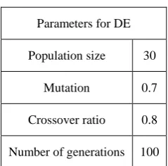
The parameter selection plays an important role in convergence of the algorithm. The control parameter setting for a DE algorithm with DE/rand/1/binary strategy is as given in Table 3.
Table 3. Parameter selection
Parameters for DE
Population size 30
Mutation 0.7
Crossover ratio 0.8
Number of generations 100
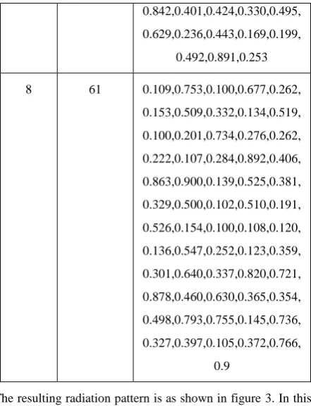
[image:4.595.56.284.69.252.2]Now ring radii, element amplitude excitations are also optimized in addition to thinning. Table 4 shows the optimum radii and Table 5 shows the ON/OFF status for the 8 ring concentric array. The optimized element excitations in each ring are presented in Table 6.
Table 4. Optimum Ring radii for M=8 rings
Ring number Radius Number of elements
in each ring
1 0.6629 8
2 1.3441 16
3 1.8695 23
4 2.5521 32
5 3.1786 39
6 3.6981 46
7 4.2538 53
[image:4.595.326.529.82.631.2]8 4.8632 61
Table 5. Element status for M=8 rings
Ring number
Number of elements in
each ring
Thinning weights (1=ON. 0=OFF)
1 8 1,1,0,1,0,0,0,0,
2 16 0,1,1,1,1,0,0,0,1,0,1,1,
0,0,0,1,
3 23 1,0,0,1,1,1,1,1,0,1,1,1,
0,1,1,0,1,1,1,1,0,1,0,
4 32 1,1,0,0,1,1,1,0,0,1,1,0,
1,1,0,0,0,0,1,0,1,1,1,0,
1,1,0,1,0,1,0,0,
5 39 1,0,0,0,0,1,1,1,0,1,0,0,
1,0,1,1,1,1,1,1,0,1,0,1,
1,1,0,1,1,0,1,1,1,0,1,0,
0,1,1,
6 46 0,1,1,0,0,1,1,1,1,1,0,1,
1,1,1,1,0,1,0,1,0,1,0,1,
0,1,0,1,1,1,0,0,0,1,1,1,
1,1,1,0,0,0,1,0,0,1,
7 53 1,0,0,0,0,0,0,1,0,0,1,1,
1,1,1,0,1,0,1,0,0,0,0,0,
0,0,1,0,0,1,1,1,0,1,1,0,
0,1,1,1,0,1,1,0,1,1,0,1,
0,1,1,0,1,
8 61 1,0,1,0,1,1,0,0,1,0,1,0,
1,0,0,1,1,0,0,0,1,0,1,1,
0,0,1,0,0,1,1,1,1,1,0,1,
0,1,1,0,0,1,1,1,1,1,0,0,
1,0,1,1,0,1,0,1,1,1,0,0,1
Table 6. Amplitude excitations for M=8 rings
Ring number
Number of elements in each ring
Element excitations
1 8 0.774,0.697,0.504,0.853,0.815,
0.802,0.610,0.900
2 16 0.873,0.289,0.628,0.824,0.383,
0.239,0.722,0.610,0.863,0.641,
-1 -0.8 -0.6 -0.4 -0.2 0 0.2 0.4 0.6 0.8 1
-50 -45 -40 -35 -30 -25 -20 -15 -10 -5 0
u
E
(u
)
i
n
d
[image:4.595.107.227.329.447.2] [image:4.595.76.256.521.754.2]0.884,0.354,0.713,0.845,0.869,
0.641
3 23 0.174,0.446,0.190,0.103,0.437,
0.222,0.383,0.495,0.733,0.340,
0.621,0.395,0.475,0.565,0.721,
0.137,0.378,0.762,0.900,0.302,
0.900,0.547,0.261
4 32 0.887,0.900,0.447,0.186,0.720,
0.104,0.533,0.513,0.549,0.431,
0.389,0.707,0.573,0.675,0.893,
0.655,0.101,0.706,0.171,0.100,
0.349,0.802,0.399,0.348,0.888,
0.347,0.767,0.323,0.601,0.574,
0.900,0.494
5 39 0.736,0.160,0.871,0.900,0.735,
0.254,0.705,0.484,0.873,0.192,
0.280,0.768,0.872,0.100,0.843,
0.387,0.634,0.755,0.152,0.420,
0.834,0.899,0.862,0.452,0.309,
0.899,0.466,0.900,0.411,0.418,
0.495,0.631,0.900,0.159,0.758,
0.546,0.898,0.758,0.638
6 46 0.457,0.878,0.415,0.753,0.876,
0.365,0.296,0.883,0.524,0.809,
0.798,0.888,0.188,0.212,0.477,
0.349,0.283,0.217,0.834,0.266,
0.355,0.243,0.523,0.375,0.668,
0.556,0.240,0.549,0.134,0.219,
0.483,0.850,0.624,0.863,0.880,
0.606,0.831,0.100,0.460,0.642,
0.900,0.107,0.403,0.543,0.714,
0.186
7 53 0.418,0.895,0.616,0.900,0.131,
0.149,0.482,0.469,0.299,0.882,
0.826,0.670,0.784,0.794,0.869,
0.218,0.384,0.100,0.412,0.465,
0.443,0.380,0.740,0.785,0.857,
0.100,0.642,0.889,0.377,0.234,
0.461,0.306,0.770,0.107,0.900,
0.900,0.717,0.119,0.888,0.865,
0.842,0.401,0.424,0.330,0.495,
0.629,0.236,0.443,0.169,0.199,
0.492,0.891,0.253
8 61 0.109,0.753,0.100,0.677,0.262,
0.153,0.509,0.332,0.134,0.519,
0.100,0.201,0.734,0.276,0.262,
0.222,0.107,0.284,0.892,0.406,
0.863,0.900,0.139,0.525,0.381,
0.329,0.500,0.102,0.510,0.191,
0.526,0.154,0.100,0.108,0.120,
0.136,0.547,0.252,0.123,0.359,
0.301,0.640,0.337,0.820,0.721,
0.878,0.460,0.630,0.365,0.354,
0.498,0.793,0.755,0.145,0.736,
0.327,0.397,0.105,0.372,0.766,
0.9
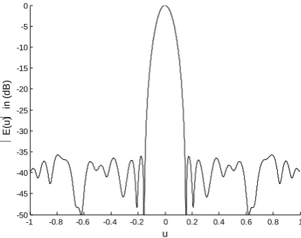
[image:5.595.320.541.70.358.2]The resulting radiation pattern is as shown in figure 3. In this case, a peak SLL of -34.56dB is obtained which shows a further improvement of around 3.5dB compared to previous case.
Figure 3. Radiation pattern for M=8 rings (both radii and element amplitudes optimized)
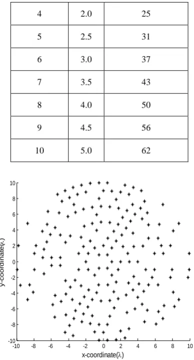
Similarly for 10 ring concentric circular array, Table 7 shows the ring radii and the organization of ON elements is shown in figure 4.
Table 7. Ring radii for M=10 rings
Ring number Radius Number of elements
in each ring
1 0.5 6
2 1.0 12
3 1.5 18
-1 -0.8 -0.6 -0.4 -0.2 0 0.2 0.4 0.6 0.8 1
-50 -45 -40 -35 -30 -25 -20 -15 -10 -5 0
u
E
(u
)
i
n
(
d
B
[image:5.595.318.541.398.567.2]4 2.0 25
5 2.5 31
6 3.0 37
7 3.5 43
8 4.0 50
9 4.5 56
10 5.0 62
Figure 4. Element Status for M=10 rings
[image:6.595.67.262.70.431.2]The far field pattern is shown in figure 5. A PSLL of -33.39dB is obtained for only thinning case.
Figure 5. Radiation pattern for M=10 rings
Optimum ring radii for case two are listed in Table 8 and figure 6 shows the layout of ON elements. Figure 7 depicts the element excitations.
Table 8. Optimum ring radii for M=10 rings
Ring number Radius Number of elements
in each ring
1 0.581 7
2 1.172 14
3 1.684 21
4 2.276 28
5 2.839 35
6 3.349 42
7 3.876 48
8 4.431 55
9 5.027 63
[image:6.595.327.527.90.542.2]10 5.623 70
Figure 6. Element Status for M=10 rings
Figure 7. Amplitude excitations for M=10 rings
-10 -8 -6 -4 -2 0 2 4 6 8 10
-10 -8 -6 -4 -2 0 2 4 6 8 10
x-coordinate()
y-co
o
rd
in
a
te
(
)
-1 -0.8 -0.6 -0.4 -0.2 0 0.2 0.4 0.6 0.8 1
-50 -45 -40 -35 -30 -25 -20 -15 -10 -5 0
u
E
(u
)
i
n
d
B
-6 -4 -2 0 2 4 6
-6 -4 -2 0 2 4 6
x-coordinate()
y-co
o
rd
in
a
te
(
)
-6 -4
-2 0
2 4
6
-6 -4 -2 0 2 4 6
0 0.5 1
x-coordinate() y-coordinate()
A
m
p
li
tu
d
e
E
xci
ta
ti
o
[image:6.595.56.283.483.682.2]Figure 8 shows the corresponding radiation pattern. A PSLL of -35.75dB is obtained in this case. An improvement of around 2.36dB can be observed.
Figure 8. Radiation pattern for M=10 rings (both radii and element amplitudes optimized)
The comparison of Peak SLLs obtained for 8 and 10 rings for both considered cases using DE is presented in Table 9 for the sake of convenience.
Table 9. Comparison of PSLL obtained using DE and GA
Case1: Thinning only
M=8 M=10
-31.0793dB
59.009%
-33.3970dB
55.2941%
Case 2: Thinning and Variable Element Amplitudes and variable
radii
M=8 M=10
-34.5645dB
56.1151%
-35.7562dB
55.0914%
The table also lists the percentage of thinning values for both ring configurations for the considered two cases. Percentage of thinning is defined as follows:
% of thinning= (Number of ON elements/ Total number of elements)*100
From the results, it can be seen that the second method where ring radii and element excitations are both optimized in addition to thinning, resulted not only in low side lobe levels but also a reduction in percentage of thinning. That means better PSLL values are achieved even after removal of certain elements through second method. The programming is done in Matlab Language and the algorithm is run for 100 generations in each run.
5.
CONCLUSIONS
The paper presents the synthesis of low sidelobe patterns from concentric circular arrays. Two cases are considered. In the first case, the arrays are only thinned. In the second case, the ring radii and element amplitudes are also optimized in addition to array thinning. Results are presented for 8, 10 ring
concentric arrays. Results clearly show that the second case resulted in lower sidelobe levels while keeping the number of active elements minimum. The percentage of thinning is maintained well below 60% for the second case. All the optimal solutions are derived by employing a Differential Evolution Algorithm. All results are simulated using Matlab software. The work can be extended to non-isotropic elements and to different geometries.
6.
REFERENCES
[1] G.S.N.Raju, 2005. Antennas and Propagation, Pearson Education.
[2] C. A. Ballanis, 1997. Antenna theory analysis and design, 2nd edition, John Willey and Son's Inc., New York.
[3] M.T.Maa, 1974. Theory and Application of Antenna Arrays, John Wiley & Sons, Inc.
[4] P.Ioannides and C.A. Balanis, 2004. ―Uniform Circular Arrays for Smart Antennas,‖ IEEE Trans. Antennas and Propagat. Society International Symposium, Monterey, CA, Vol. 3, pp. 2796-2799, June.
[5] C. Stearns and A. Stewart, 1965. ―An investigation of concentric ring antennas with low sidelobes,‖ IEEE Transactions on Antennas and Propagation, Vol. 13, no. 6, pp. 856–863, November.
[6] N. Goto and D.K. Cheng, 1970. "On the synthesis of concentric-ring," IEEE Proceedings, Vol. 58, no. 5, pp. 839- 840, May.
[7] L. Biller and G. Friedman, 1973. ―Optimization of radiation patterns for an array of concentric ring sources,‖ IEEE Trans. Audio Electroacoustics, Vol. 21, no.1, pp. 57–61, February.
[8] M D. A. Huebner, 1978. ―Design and optimization of small concentric ring arrays,‖ In Proc. IEEE AP-S Symp., pp. 455–458.
[9] Kumar, B. P., and G. R. Branner, 1999. ―Design of low sidelobe circular ring array by element radius optimazation,‖ Proc. IEEE Antennas Propagation Int. Symp., Vol. 3, pp. 2032–2035, July.
[10]Dessouky, M., H. Sharshar, and Y. Albagory, 2006. ―Efficient sidelobe reduction technique for small-sized concentric circular array,‖ Progress In Electromagnetics Research, Vol. 65, pp. 187–200.
[11]Randy L.Haupt, 1994. ―Thinned Arrays using Genetic Algorithms,‖ IEEE Transactions on Antennas and Propagation, Vol. 42, no.7, pp. 993-999, July.
[12]Haupt, R. L., 2008. ―Thinned concentric ring arrays,‖ Proc. IEEE Antennas Propagation Int. Symp., SanDiego, CA ,pp. 1–4, July.
[13]V.Rajya Lakshmi and G.S.N.Raju, 2011. ―Optimization of Radiation Patterns of Array Antennas,‖ PIERS Proceedings, Suzhou, China, pp. 1434-1438, 12-16 September.
[14]Pathak, N., P. Nanda, and G. K. Mahanti, 2009. ―Synthesis of thinned multiple concentric circular ring array antennas using particle swarm optimization,‖ Journal of Infrared, Millimeter and Terahertz Waves, Vol. 30, no. 7, pp. 709–716, Springer, New York.
-1 -0.8 -0.6 -0.4 -0.2 0 0.2 0.4 0.6 0.8 1
-50 -45 -40 -35 -30 -25 -20 -15 -10 -5 0
u
E
(u
)
i
n
(
d
B
[image:7.595.57.277.125.299.2][15]U. Singh and T. S. Kamal, 2012. ―Synthesis of thinned planar concentric circular antenna arrays using biogeography-based optimisation,‖ IET Microwaves, Antennas and Propagation, Vol. 6, no. 7, pp. 822–829.
[16]Basu, B. and G. K. Mahanti, 2012. ―Thinning of concentric two-ring circular array antenna using fire fly algorithm,‖ Scientia Iranica, Vol. 19, no. 6, pp. 1802– 1809, Dec.
[17]R. Storn, and K. Price, 1997. ―Differential evolution—A simple and efficient heuristic for global optimization over continuous spaces,‖ Journal of Global Optimization, Vol.11, no. 4, pp. 341-359.
[18]Yang, S. A. Qing, Y. B. Gan, 2003. ―Synthesis of low sidelobe antenna arrays using the differential evolution algorithm,‖ IEEE Proc, Antennas and Propagation Society International Symposium, Vol. 1, pp. 780 - 783.
[19]Panduro, M. A., C. A. Brizuela, L. I. Balderas, and D. A. Acosta, 2009. ―A comparison of genetic algorithms, particle swarm optimization and the differential evolution method for the design of scannable circular antenna arrays‖, Progress In Electromagnetics Research B, Vol. 13, pp. 171-186.
[20]D. Mandal, A. Chatterjee, and A. K. Bhattacharjee, 2013. ―Design of Fully Digital Controlled Shaped Beam Synthesis Using Differential Evolution Algorithm,‖ International Journal of Antennas and Propagation, Vol. 2013, pp. 1–9.
[21]Kenneth V.Price, Rainer M. Storn, Jouni A. Lampinen, 2005. Differential Evolution: A Practical Approach to Global Optimization, Springer.
[22]R. L. Haupt, 2008. ―Optimized element spacing for low sidelobe concentric ring arrays,‖ IEEE Trans. Antennas Propag., Vol. 56, no.1, pp. 266–268, January.
7.
AUTHOR’S PROFILE
G.S.K.Gayatri Devi received her Bachelor of Technology degree in Electronics and Communication Engineering in the year of 2006 from JNTU Hyderabad and the Master of Engineering in Electronic Instrumentation in 2008 from
Andhra University College of Engineering (A). Currently, she is working towards her Ph.D degree in the Department of Electronics and Communication Engineering, Andhra University College of Engineering (A). Her Research interests include Array Antenna Design, EMI/EMC, Soft Computing. She is a life member of SEMCE (India).
Dr. G.S.N. Raju received his B.E., M.E. with distinction and first rank from Andhra University and Ph.D. from IIT, Kharagpur. At present, he is the Vice – Chancellor of Andhra University and a Senior Professor in Electronics and Communication Engineering. He is in teaching and research for the last 30 years in Andhra University. He guided 28 Ph.D.s in the fields of Antennas, Electromagnetics, EMI/EMC and Microwave, Radar Communications, Electronic circuits. Published about 304 technical papers in National/ International Journals/ Conference Journals and transactions. He is the recipient of ‗The State Best Teacher Award‘ from the Government of Andhra Pradesh in 1999, ‗The Best Researcher Award‘ in 1994, ‗Prof. Aiya Memorial National IETE Award‘ for his best Research guidance in 2008 and Dr. Sarvepalli Radhakrishnan Award for the Best Academician of the year 2007, He was a visiting Professor in the University of Paderborn and also in the University Karlsruhe, Germany in 1994. He held the positions of Principal, Andhra University College of Engineering (A), Visakhapatnam, Chief Editor of National Journal of Electromagnetic Compatibility. Prof. Raju has published five textbooks Antennas and Wave Propagation, Electromagnetic Field Theory and Transmission Lines, Electronics Devices and Circuits, Microwave Engineering, Radar Engineering and Navigational Aids. Prof. Raju has been the best faculty performer in Andhra University with the performance index of 99.37%.