Dynamics of coupled bosonic systems with applications to preheating

Dynamics of coupled bosonic systems with applications to preheating

Daniel Cormier

Centre for Theoretical Physics, University of Sussex, Falmer, Brighton, BN1 9QH, United Kingdom

Katrin Heitmann*

T-8, Theoretical Division, Los Alamos National Laboratory, Los Alamos, New Mexico 87545

Anupam Mazumdar

The Abdus Salam International Centre for Theoretical Physics, Strada Costiera, I-10, 34100 Trieste, Italy

共Received 22 May 2001; published 9 April 2002兲

Coupled, multifield models of inflation can provide several attractive features unavailable in the case of a single inflaton field. These models have a rich dynamical structure resulting from the interaction of the fields and their associated fluctuations. We present a formalism to study the nonequilibrium dynamics of coupled scalar fields. This formalism solves the problem of renormalizing interacting models in a transparent way using dimensional regularization. The evolution is generated by a renormalized effective Lagrangian which incorpo-rates the dynamics of the mean fields and their associated fluctuations at one-loop order. We apply our method to two problems of physical interest:共i兲a simple two-field model which exemplifies applications to reheating in inflation, and共ii兲a supersymmetric hybrid inflation model. This second case is interesting because inflation terminates via a smooth phase transition which gives rise to a spinodal instability in one of the fields. We study the evolution of the zero mode of the fields and the energy density transfer to the fluctuations from the mean fields. We conclude that back reaction effects can be significant over a wide parameter range. In particular for the supersymmetric hybrid model we find that particle production can be suppressed due to these effects.

DOI: 10.1103/PhysRevD.65.083521 PACS number共s兲: 98.80.Cq

I. INTRODUCTION

In recent years, the study of nonequilibrium dynamics in quantum field theory has received much attention in various areas of physics, and particularly in cosmology. The work has been driven largely by inflation关1兴, the most successful known mechanism for explaining the large-scale homogene-ity and isotropy of the universe and the small-scale inhomo-geneity and anisotropy of the Universe 关2兴. With observa-tions for the first time able to directly test the more detailed predictions of specific inflationary models, the efforts in un-derstanding inflation and its dynamics have redoubled.

One area of particular interest is the dynamics of multi-field models of inflation in which the inflaton is coupled to another dynamical field during inflation. These models can lead to a variety of features unavailable in the case of a single field. Such multifield scenarios include the well known hybrid inflation models关3兴.

On top of the dynamics during inflation, the subsequent phase of energy transfer between the inflaton and other de-grees of freedom leading to the standard picture of big bang cosmology has been the subject of intense study. The inflaton may decay through perturbative processes 关4,5兴 as well as nonperturbative parametric amplification关6,7兴. The latter can lead to explosive particle production and very efficient re-heating of the universe.

Hybrid inflation and reheating models share an important common thread. They both involve the coupling of two or more dynamical, interacting scalar fields 共or higher spin

fields关8兴兲. An important aspect of such systems is the possi-bility of mixing between the fields. In Ref. 关9兴for example the classical inflaton decay is investigated for a two field model by solving the non-linear equations of motions on a grid. In Ref. 关10兴, the authors treat the problem of coupled quantum scalar and fermion fields at the tree level. Because of the small couplings involved in inflationary cosmology, such a tree level analysis is useful in a variety of physical situations.

However, hybrid models as well as the dynamics of re-heating typically include processes such as spinodal decom-position 关11,12兴 and parametric amplification which require one to go beyond the tree level by including quantum effects either in a perturbative expansion or by means of nonpertur-bative mean field techniques such as the Hartree approxima-tion or a large-N expansion关5,13,14兴.

Going beyond tree level brings in the issue of renormal-ization. The problem of renormalization of time evolution equations in single field models was understood several years ago. In one of the first papers in this field, Cooper and Mottola showed in 1987 Ref.关15兴, that it is possible to find a renormalization procedure which leads to counter terms independent of time and initial conditions of the mean field. They used a WKB expansion in order to extract the diver-gences of the theory. In a later paper Cooper et al. also dis-cussed a closely related adiabatic method in order to renor-malize the ␾4 theory in the large-N approximation. Also Boyanovsky and de Vega, Ref.关11兴, used a WKB method in order to renormalize time-dependent equations in one-loop order, and later on Boyanovsky et al.关12兴investigated a␾4 model in the large-N approximation and the Hartree approxi-mation, too. In 1996 Baacke et al., Ref. 关16兴, proposed a slightly different method in order to extract the divergences

*On leave of absence from Dortmund University, Dortmund,

of the theory, which enabled them to use dimensional regu-larization. In contrast to the WKB ansatz this method can be extended for coupled system, which was demonstrated in Ref.关17兴. This procedure will be used also in this paper. We work in the context of a closed time path formalism 关18兴 appropriate to following the time-dependent evolution of the system. In this formalism, the in-vacuum plays a predomi-nant role, as quantities are tracked by their in-in expectation values 共in contrast to the in-out formalism of scattering theory兲. We construct the in-vacuum by diagonalizing the mass matrix of the system at the initial time t⫽0. However, because of the time-dependent mixing, a system initially di-agonalized in this way will generally not be didi-agonalized at later times.

One approach to this problem, taken in Ref. 关10兴, is to diagonalize the mass matrix at each moment in time through the use of a time-dependent rotation matrix. The cost of do-ing so is the appearance of time derivatives of the rotation matrix into the kinetic operators of the theory. While such a scheme is in principle workable beyond the tree level, the modified kinetic operators introduce complications into the extraction of the fluctuation corrections as well as the diver-gences that are to be removed via renormalization.

We take an alternative approach where the mass matrix is allowed to be non-diagonal for all times t⬎0 and account for the mixing by expanding each of the fields in terms of all of the in-state creation and annihilation operators. The cost of doing so in an N-field system is the need to track N2complex mode functions representing the fields instead of the usual N. However, this allows standard techniques to be used to prop-erly renormalize the system. For the two-field systems com-mon in inflationary models, this effective doubling of the field content adds a relatively minor cost.

For simplicity and clarity, we will work in Minkowski spacetime and in a one-loop approximation. Extensions both to Friedmann-Robertson-Walker spacetimes and to simple non-perturbative schemes such as the Hartree approximation, while more complicated than the present analysis, present no fundamental difficulties. We note that Minkowski spacetime is a good approximation in the latter stages of certain hybrid inflation models, and it will also allow comparison with much of the original reheating literature 关4 – 6兴 which often neglects the effects of expansion, allowing us to directly de-termine the role played by the mixing of the fields in the dynamics.

The outline of the paper is as follows. We begin by con-sidering the Lagrangian for N coupled scalar fields and set up our formalism for the quantization of the system. This is followed by an outline of the renormalization procedure. We then provide a summary of the results for the two-field case. We demonstrate the formalism with two examples: a simple reheating model and a hybrid inflation model motivated by supersymmetry.

In the reheating model we investigate two relevant re-gimes discussed in detail in the literature关6,7兴, viz., the nar-row resonance regime and the broad resonance regime. These different regimes occur depending on the choice of initial conditions. Usually in these models the mixing effects of the fields were neglected by choosing a vanishing initial

value for one of the mean fields: We are now able to treat the full system and to investigate these mixing effects. For this purpose we concentrate on studying the behavior of the fluc-tuation integrals for the different fields and the time-dependent mixing angle. Depending on the regime, as the mean fields evolve, the effects of the mixing can be quite different. In the narrow resonance regime the mixing angle is very small and plays a subdominant role, whereas in the broad resonance regime the mixing effects are very impor-tant. Therefore, we emphasize that neglecting the mixing could lead to incomplete results.

Supersymmetric hybrid models are a special realization of general hybrid inflationary models共see, e.g., Refs.关19,20兴兲. Based on a softly broken supersymmetry potential, the spe-cial feature of these models is the occurrence of only one coupling constant, whereas in nonsupersymmetric hybrid models there are at least two different couplings. Thus, in the supersymmetric case there is only one natural frequency of oscillation for the mean fields as long as fluctuations are neglected. This leads to efficient particle production during the preheating stage in the early universe. However, we show below that, by taking into account the fluctuations and inves-tigating the full mixed system, this feature of supersymmet-ric hybrid models can be lost in some regimes. This is be-cause the effective mass corrections for the two fields are different in these regimes, which leads to a chaotic trajectory for the renormalized field equations of motion in a phase space which mimics the situation of a nonsupersymmetric hybrid model. It appears, then, that supersymmetric hybrid models can lose some of their attractiveness compared to general hybrid models.

II. N FIELDS

We work with the following Lagrangian for real scalar fields ⌽iwith i⫽1 . . . N:

L关⌽i兴⫽

兺

i⫽1 N

1

2⳵␮⌽i共x兲⳵

␮_⌽

i共x兲⫺V关⌽i共x兲兴, 共2.1兲

where the potential is

V共⌽_i兲⫽

兺

i, j,k,l⫽1

N

A_i⌽_i⫹1

2mi j⌽i⌽j⫹ 1

3!gi jk⌽i⌽j⌽k

⫹_4!1 ␭i jkl⌽i⌽j⌽k⌽l. 共2.2兲

Note that mi j, gi jk, and␭i jkl are symmetric in each index, but are generally non-diagonal resulting in the mixing of the different fields. In what follows, subscripts and superscripts i . . . n run over the values 1 . . . N and we use a convention in which summation is assumed over repeated lowered indi-ces, but not raised indices.

We will expand each field about their expectation values 共taken to be space translation invariant兲:

Expanding the equations of motion and keeping terms to quadratic order in the fluctuations yields a one-loop approxi-mation. The equations of motion for the zero modes ␾i are determined via the tadpole condition. We have

␾¨

i⫹Ai⫹mi j␾j⫹ 1

2gi jk␾j␾k⫹ 1

6␭i jkl␾j␾k␾l

⫹1₂gi jk

具

␦␾j␦␾k

典⫹

1

2␭i jkl␾j

具

␦␾k␦␾l

典⫽

0. 共2.4兲 To this order, the fluctuations obey the equation

␦¨_␾

i⫺ⵜជ2␦␾i⫹Mi j␦␾j⫽0, 共2.5兲 with the mass matrix

Mi j⫽mi j⫹gi jk␾k⫹ 1

2␭i jkl␾k␾l. 共2.6兲 As indicated in the Introduction, the complication that arises is not the fact that the mass matrix共2.6兲contains mix-ing between the various fields, rather that the mixmix-ing changes with time as the␾ievolve according to Eq.共2.4兲. This means that if we diagonalize the mass matrix at one time, it will not generally be diagonal at any other time.

Nonetheless, it is most convenient to quantize in terms of a diagonal system at the initial time t⫽0. We define the matrix

Di j⫽OikMklOl j T

, 共2.7兲

and the corresponding fluctuation fields

Xi⫽Oi j␦␾j, 共2.8兲 whereO_{i j}is an orthogonal rotation matrix.D_{i j}is diagonal at the initial time:

Di j⫽Di␦i j, 共2.9兲

without summation over the raised index i. The Xi obey the equations of motion

X¨_i⫺ⵜជ2_X

i⫹Di jXj⫽0. 共2.10兲 We quantize the system by defining a set of creation and annihilation operators a_␣†(kជ) and a_␣(kជ) where ␣⫽1 . . . N corresponds to the in-state quanta of frequency

␻␣⫽

冑

k2⫹D␣. 共2.11兲

As the mixing changes in time, each of the fields X_i is ex-panded in terms of all of the in-state operators. We have

Xi⫽

兺

␣⫽1 N

冕

d3k 共2␲兲3

1

2␻_␣0关a␣共ជk兲Ui␣共kជ,t兲e ikជ•xជ

⫹a_␣†共kជ兲Ui␣*共kជ,t兲e⫺ik

ជ_•xជ_{兴. 共2.12兲}

The initial conditions for the N2complex mode functions are

U_i␣共kជ,0兲⫽␦i␣, U˙_i␣共ជk,0兲⫽⫺i␻_␣U␣_i共kជ,0兲. 共2.13兲 It is convenient to define the fluctuation integrals

具

X_iX_j

典

⫽

兺

␣⫽1

N

冕

d3k 共2␲兲3

1 2␻_␣0

U_i␣*_共kជ,t兲U_j␣共kជ,t兲, 共2.14兲 from which it is straightforward to determine the contribu-tions appearing in the zero mode equacontribu-tions 共2.4兲:

具

␦␾i␦␾j

典

⫽Oik T_O

jl T

_具

_X

iXj

典

. 共2.15兲 It will also prove convenient to introduce the rotated cou-plings

Gi jk⫽gilmOl j T_O

mk T

, 共2.16兲

⌳i jkl⫽␭i jmnOmk

T _O

nl T

, 共2.17兲

which allows us to write the zero mode equations as

␾¨

i⫹Ai⫹mi j␾j⫹ 1

2gi jk␾j␾k⫹ 1

6␭i jkl␾j␾k␾l

⫹1₂Gi jk

具

XjXk

典⫹

1

2⌳i jkl␾j

具

XkXl

典

⫽0, 共2.18兲 while the mode functions obey the equations

U¨_i␣共kជ,t兲⫹共k2⫹Di j兲Uj␣共kជ,t兲⫽0. 共2.19兲 In addition to the equations of motion, it is useful to have an expression for the energy density of the system. This is particularly true when one completes numerical simulations of the system, since energy conservation is a powerful check of the accuracy of the simulations. After once again decom-posing the fields into their expectation values and fluctua-tions, the energy density to one loop order is

E⫽1

2␾˙i

2_⫹Ai␾i⫹1

2mi j␾i␾j⫹ 1

3!gi jk␾i␾j␾k

⫹_4!1 ␭i jkl␾i␾j␾k␾l⫹1₂

具

X˙_i2

典

⫹1₂

具

共ⵜជXi兲2

典⫹

1

2Di j

具

XiXj

典

, 共2.20兲 where we have defined the integrals

具

X˙i

典⫽

兺

␣⫽1 N

冕

d3_k 共2␲兲3

1 2␻_␣0兩

U˙_i␣共kជ,t兲兩2, 共2.21兲

具

共ⵜជXi兲2

典⫽

兺

␣⫽1 N

冕

d3_k 共2␲兲3

k2

2␻_␣0兩

U_i␣共kជ,t兲兩2.

A. Divergence structure and renormalization

The mode integrals in the equation of motion defined by Eq. 共2.14兲and in the energy density defined by Eqs. 共2.21兲, 共2.22兲are divergent and have to be regulated, allowing for a renormalization of the theory. We require a method of ex-tracting the divergent terms appearing in the mode integrals, a nontrivial task, since the mode equations vary in time and they are coupled. Our aim is now to find counter terms, which are independent of the initial value of the mean fields in order to formulate a finite theory. The correct choice of the initial condition for the fluctuations guarantees that the theory is renormalizable. One way to extract the divergences of the mode integrals is due to a WKB method which allows for a high momentum expansion of the mode functions. However, when the fields are coupled, as in the present case, the usual formulation of the WKB expansion runs into diffi-culties which are yet to be resolved.

An alternative method has been developed 关16,17,21兴 which relies on a formal perturbative expansion in the effec-tive masses and time derivaeffec-tives of the masses of the fields. As such, it results in a series expansion of the mode func-tions in powers of m/␻ and m˙ /␻2, etc. The first few terms in the series include the divergent parts of the integrals that are to be removed via renormalization.

We begin by introducing the following ansatz for the mode functions:

U␣_j⫽e⫺i␻␣0t共␦ j

␣_⫹f

j

␣_{兲. 共2.23兲}

The first term on the right-hand side anticipates a quadratic divergence in the quantities

具

X_i2

典

. We define the following potential:

V_{i j}␣共t兲⫽D_{i j}共t兲⫺D␣␦i j. 共2.24兲

The equations of motion for the mode functions Eqs.共2.19兲 can be written in a suggestive form with the help of Eqs. 共2.23兲,共2.24兲

f¨_j␣⫺i2␻_␣0f˙␣j⫽⫺

兺

l⫽1,2

V_jl␣共␦_l␣⫹f_l␣兲. 共2.25兲

The terms on the right-hand side of this expression are treated as perturbations to write the f

⬘

s order by order in V, with the initial conditions fi_j(0)⫽f˙_ji(0)⫽0. To first order in V, we have the equations of motion:

f¨␣_j(1)⫺2i␻_␣0f˙␣j

(1)_⫽⫺V j␣

␣ _{. 共2.26兲}

The corresponding integral solutions for the real part of the f ’s are

2Rf_j␣(1)⫽⫺ V␣j ␣

2␻_␣0

⫹

冕

0 t

dt

⬘

V ˙

␣j

␣_共t

_⬘

_兲

2␻_␣0

cos共2␻_␣0t

⬘

兲, 共2.27兲

while the imaginary part is of order 1/␻3 and does not con-tribute to the divergences关17兴.

Using these results, we find quadratic and logarithmic di-vergences:

具

XiXj

典

div⫽

冕

d3k 共2␲兲3

冉

1 2␻_j␦i j⫺

1 4␻3_jVi j

j

冊

, 共2.28兲

which must be removed via some renormalization procedure while also providing finite corrections to the parameters of the theory.

To make the renormalization scheme explicit, we adopt dimensional regularization. We define the following diver-gent integrals:

冕

d3k 共2␲兲3

1

2

冑

k2⫹␮2⫽⫺␮ 2_I

⫺3共␮兲⫺ ␮2

16␲2, 共2.29兲

冕

d3k 共2␲兲3

1

4共k2⫹␮2兲3/2⫽I⫺3共␮兲, 共2.30兲 where␮is an arbitrary renormalization point and I_⫺3carries the infinite contributions. In dimensional regularization I_⫺3(␮) is given by

I_⫺3共␮兲⫽ 1 16␲2

再

2 ⑀⫹ln

4␲␮2

m2 ⫺␥

冎

. 共2.31兲 The infinite part of

具

X_iX_j

典

is found to be simply

具

XiXj

典

infinite⫽⫺Di jI⫺3共␮兲. 共2.32兲

This leads to mass and coupling constant counterterms of the following form

␦Ai⫽ 1

2I⫺3共␮兲gi jkmjk, 共2.33兲

␦mi j⫽ 1

2I⫺3共␮兲关gikmgkm j⫹␭i jklmkl兴, 共2.34兲

␦gi jk⫽ 3

2I⫺3共␮兲gilm␭lm jk, 共2.35兲

␦␭i jkl⫽ 3

2I⫺3共␮兲␭i jmn␭mnkl. 共2.36兲 It is important to notice that these counterterms are indepen-dent of the initial conditions of the mean fields ␾i.

In addition to these counterterms, there are finite correc-tions of the parameters coming from the finite parts of the integrals共2.28兲:

具

XiXj

典

div,finite⫽⫺ 1 16␲2D

j_␦ i j⫺

1 16␲2Di jln

Dj

␮2. 共2.37兲

⌬Ai⫽⫺ 1

32␲2

冋

Gi j jD j_⫹g

i jkmjkln Dk

␮2

册

, 共2.38兲

⌬mi j⫽⫺ 1

32␲2

冋

⌳i jkkD k_⫹共g

iklgkl j⫹␭i jklmkl兲

⫻lnD k

␮2

册

, 共2.39兲

⌬gi jk⫽⫺ 1

8␲2gilm␭lm jkln Dm

␮2, 共2.40兲

⌬␭i jkl⫽⫺ 3

32␲2␭i jmn␭mnklln Dm

␮2. 共2.41兲

These finite corrections are also contributing to the energy density. In addition we find a finite part due to the cosmo-logical constant renormalization.

The full, finite equations of motion become

␾¨

i⫹Ai⫹⌬Ai⫹共mi j⫹⌬mi j兲␾j

⫹1

2共gi jk⫹⌬gi jk兲␾j␾k

⫹1₆共␭i jkl⫹⌬␭i jkl兲␾j␾k␾l

⫹1

2共Gikl⫹⌳i jkl␾j兲_␣

兺

_⫽1 N

冕

d3k 共2␲兲3

1 2␻_␣0

⫻

冋

f_k␣*f_l␣⫹␦_k␣f_l␣⫹␦_l␣f_k␣*⫹ 1 2␻_␣2₀␦l

␣_V

k␣

␣

册

_⫽0.

共2.42兲

B. Two fields

The two-field case is often encountered, and the physical applications we present in the next section are both in this category. It is therefore worthwhile to pause to look at a few details of such systems. We begin with a system of two real scalar fields ⌽and X

L⫽1

2共⳵␮⌽兲 2_⫹1

2共⳵␮X兲

2_{⫺V共⌽,X兲, 共2.43兲}

with the potential

V共⌽,X兲⫽1 2m␾

2_⌽2_⫹1 2m␹

2 X2⫹ ␭

4!⌽ 4_⫹ ␬

4!X 4

⫹g

2

4 ⌽

2_X2_{. 共2.44兲}

This Lagrangian has the same form as that studied in the preceding section with the identifications

⌽1⬅⌽, ⌽2⬅X,

m₁₁⬅m_␾2, m₂₂⬅m_␹2, m₁₂⫽m₂₁⫽0,

␭1111⬅␭, ␭2222⬅␬, ␭1122⬅g2,

␭1112⫽␭1222⫽0,Ai⫽0, gi jk⫽0. 共2.45兲

The remaining components of ␭i jkl are determined by the fact that it is symmetric in each of its indices.

The mass matrix Mis

M⫽

冉

m␾

2_⫹␭␾2_/2⫹g2_␹2_{/2 g}2_␾␹

g2␾␹ m_␹2⫹␬␹2/2⫹g2␾2/2

冊

. 共2.46兲

For two fields, the orthogonal rotation matrix can be written in terms of a single mixing angle␪. The matrix has the form

O⫽

冉

_⫺cos␪ sin␪

sin␪ cos␪

冊

, 共2.47兲 where the mixing angle is determined by the t⫽0 mass ma-trixM, Eq.共2.46兲, through the relation

tan␪⫽ 1

2M12共0兲 关M22共

0兲⫺M11共0兲

⫹

冑

关M22共0兲⫺M11共0兲兴2⫹4M12 2

共0兲兴. 共2.48兲

The eigenvalues ofOare the diagonal elements of the matrix D, Eq.共2.7兲, at the initial time:

D共0兲⫽

冉

D1 0

0 D2

冊

, 共2.49兲

with the values

D1⫽1

2关M11共0兲⫹M22共0兲

⫹

冑

关M22共0兲⫺M11共0兲兴2⫹4M12

2 _{共0兲兴, 共2.50兲}

D2⫽1

2关M11共0兲⫹M22共0兲

⫺

冑

关M22共0兲⫺M11共0兲兴2⫹4M12 2

共0兲兴. 共2.51兲

D共t兲⫽

冉

c_␪2M11⫹2s␪c␪M12⫹s␪ 2_M

22 s␪c␪M22⫺s␪c␪M11⫹共c␪ 2_⫺

s_␪2兲M12 s_␪c_␪M22⫺s␪c␪M11⫹共c_␪

2_⫺

s_␪2兲M12 ⫺2c_␪ 2_M

22⫺2s␪c␪M12⫹s_␪ 2_M

11

冊

共2.52兲

The zero mode equations, before renormalization, read ␾¨_⫹m

␾

2_␾⫹␭ 6␾

3_⫹g 2

2 ␾␹ 2_⫹

兺

i j

Qi j共t兲

具

XiXj

典⫽

0, 共2.53兲

␹¨_⫹m ␹

2_␹⫹␬ 6␹

3_⫹g 2

2 ␹␾ 2_⫹

兺

i j

Ri j共t兲

具

XiXj

典⫽

0, 共2.54兲

where

Qi j⫽⌳1ki j␾k

⫽

冉

␭ 2c␪

2 ␾⫹g

2

2 s␪ 2

␾⫹g2s_␪c_␪␹ ⫺␭

2s␪c␪␾⫹ g2

2 s␪c␪␾⫹ g2

2 共c␪ 2_⫺

s_␪2兲␹

⫺␭₂s_␪c_␪␾⫹g 2

2 s␪c␪␾⫹ g2

2 共c␪ 2_⫺

s_␪2兲␹ ␭ 2s␪

2_␾⫹g 2

2 c␪ 2_␾⫺

g2s_␪c_␪␹

冊

,

R_{i j}⫽⌳2ki j␾k

⫽

冉

␬ 2s␪

2_␹⫹g 2

2 c␪ 2_␹⫹

g2s_␪c_␪␾ ␬

2s␪c␪␹⫺ g2

2 s␪c␪␹⫹ g2

2 共c␪ 2_⫺

s_␪2兲␾ ␬

2s␪c␪␹⫺ g2

2 s␪c␪␹⫹ g2

2 共c␪ 2_⫺

s_␪2兲␾ ␬ 2c␪

2_␹⫹g 2

2 s␪ 2_␹⫺

g2s_␪c_␪␾.

冊

. 共2.55兲

The total energy density of the system, including the fluc-tuations, can be expressed as

E⫽1

2␾˙ 2_⫹1

2␹˙ 2_⫹1

2m␾ 2_␾2_⫹1

2m␹ 2_␹2_⫹ ␭

4!␾ 4_⫹ ␬

4!␹ 4

⫹g

2

4 ␾ 2_␹2_⫹1

2

具

X˙i 2

_典⫹

1

2

具

共ⵜជXi兲 2

_典⫹

1

2Di j

具

XiXj

典

. 共2.56兲

Now we have to formulate finite equations of motion and a finite energy density. We adopt the renormalization proce-dure of Sec. II A for the N field case. By using the identifi-cations共2.45兲we derive the appropriate counterterms for the two field case from Eqs.共2.33兲–共2.36兲. We find in particular

␦m_␾2⫽1 2共␭m␾

2_⫹

g2m_␹2兲I_⫺3共␮兲,

␦m_␹2⫽1 2共g

2_m

␾

2_⫹␬m

␹

2_兲I

⫺3共␮兲,

␦␭⫽3₂共␭2_⫹g4_兲I

⫺3共␮兲,

␦g2⫽g 2

2 共␭⫹␬⫹4g 2_兲I

⫺3共␮兲,

␦␬⫽3

2共g 4_⫹␬2_兲I

⫺3共␮兲. 共2.57兲

Of course we get also similar results to Eqs.共2.38兲–共2.41兲 in the N field case finite corrections to the masses and cou-plings of the form

⌬m_␾2⫽⫺ 1 32␲2兵D

1_共␭c

␪

2_⫹g2_s

␪

2_兲⫹D2_共␭s

␪

2_⫹g2_c

␪

2_兲

⫹g2_m

␹

2_L 1⫹␭m␾

2_{L2其, 共2.58兲}

⌬m_␹2⫽⫺ 1 32␲2兵D

1_共␬s

␪

2_⫹

g2c_␪2兲⫹D2共g2s_␪2⫹␬c_␪2兲

⫹g2m_␾L2⫹␬m_␹ 2

L1其, 共2.59兲

⌬␭⫽⫺ 1

32␲2兵␭ 2_L

2⫹g4L1其, 共2.60兲

⌬g2⫽⫺ 3 32␲2

再

g

4_共L

1⫹L2兲⫹ 1 2g

2_␭L 2⫹

1 2g

2_␬L 1

冎

, 共2.61兲

⌬␬⫽⫺ 1

32␲2兵g 4_L

2⫹␬2L1其, 共2.62兲

L1⫽s␪ 2

lnD 1

␮2⫹c␪ 2

lnD 2

␮2,

L2⫽s_␪ 2

lnD 2

␮2⫹c␪ 2

lnD 1

␮2. 共2.63兲

As a result of these finite corrections Eqs.共2.58兲–共2.62兲, the total Lagrangian Eq. 共2.43兲is also modified. This is exactly the renormalized Lagrangian which we needed. We also find an additional finite contribution to the classical Lagrangian given by

⌬L⫽⫺g

2_s

␪c␪␾␹

64␲2

再

4共D 1_⫺D2_兲

⫹lnD 1

D2关共␭⫹g

2_兲␹2_{⫹共␬⫹g}2_兲␾2

⫹2共m_␹2⫹m_␾2兲兴

冎

, 共2.64兲

and, the final zero mode equations for␾ and␹ are given by

␾¨_⫹共m ␾

2_⫹⌬m

␾

2_兲␾⫹1

6共␭⫹⌬␭兲␾ 3_⫹1

2共g

2_⫹⌬g2_兲␾␹2_⫹⳵⌬L ⳵␾

⫹

再

兺

l␣

Qll共t兲

冕

d3k 共2␲兲3

1

2␻_␣0

冉

2␦l␣Rfl l_⫹

f_l␣f_l␣*_⫹ Vll 4␻_␣3₀

冊

⫹

兺

␣⫽l Ql␣

冕

d3k

共2␲兲3 1 2␻_␣0

冉

Rf_l␣⫹Rf_␣␣Rf_l␣⫹If_␣␣If_l␣⫹ Vl␣

2␻_␣2₀

冊冎

⫽0, 共2.65兲 and,

␹¨_⫹共m ␾

2_⫹⌬m

␾

2_兲␹⫹1

6共␬⫹⌬␬兲␹ 3_⫹1

2共g

2_⫹⌬g2_兲␾␹2_⫹⳵⌬L ⳵␹

⫹

再

兺

l␣

Rll共t兲

冕

d3_k

共2␲兲3 1 2␻_␣0

冉

2␦_l␣Rf_ll⫹f_l␣f_l␣*_⫹ Vll 4␻_␣0

3

冊

⫹

兺

␣⫽l

Q_l␣

冕

d 3_k

共2␲兲3 1 2␻_␣0

冉

Rf_l␣⫹Rf_␣␣Rf_l␣⫹If_␣␣If_l␣⫹ Vl␣

2␻_␣2₀

冊冎

⫽0. 共2.66兲

After writing down the finite zero mode equations of mo-tion we also have to renormalize the energy density. Again by using the ansatz共2.23兲we can extract the divergent terms of the fluctuation integrals in Eq. 共2.56兲. In addition to the quadratic and logarithmic divergences we find a quartic di-vergence. This leads to a counterterm which acts as a cos-mological constant and has the form

␦⌳⫽1

4共m␹ 4_⫹m

␾

4_兲I

⫺3共m兲. 共2.67兲

Altogether the divergent part of the energy density reads

Ediv⫽⫺ I_⫺3共m兲

4

再

共g 2_m

␹

2_⫹␭

m_␾2兲␾2⫹共g2m_␾2␬m_␹2兲␹2

⫹1

2g

2_{共␭⫹␬⫹4g}2_兲␾2_␹2_⫹1 4共␭

2_⫹g4_兲␾4

⫹1

4共␬

2_⫹g4_兲␹4_⫹m

␹

4_⫹m

␾

4

冎

_{. 共2.68兲}

This expression leads of course to the same counterterms we found for the equations of motion, and therefore also to the same finite corrections to couplings and masses. Therefore it is straightforward to formulate a finite energy expression.

Now, we are in a position to discuss the physical applica-tions of our problem. This we shall do in Sec. III, but first we introduce one more quantity that is convenient in discussing the degree to which the mixing plays a role in the dynamics.

C. Time-dependent mixing angle

tan⌰共t兲⫽ 1

2M12共t兲 关M22共

t兲⫺M11共t兲

⫹

冑

共M22共t兲⫺M11共t兲兲2⫹4M12 2 _共

t兲兴. 共2.69兲

III. PHYSICAL APPLICATIONS

After setting up the technical framework, we are now in a position to investigate some relevant cosmological multi-field models for inflation. We begin our analysis with a simple two-field model often used for studying the phase of parametric amplification. 共This phase occurs just after the completion of inflation in chaotic inflationary models关6,7兴.兲 This model provides a useful context to analyze the effects due to field mixing. Next we turn our attention to a super-symmetric hybrid inflationary model, which is of particular interest in cosmology. As discussed in the literature共see, for example, Ref.关19兴兲particle production共and hence reheating兲 in these models is much more efficient compared to the non-supersymmetric hybrid models. Until now the mixing effects in these models have not been treated fully, including back reaction effects of the quantum fluctuations in the mean field approximation. This approximation does not take rescatter-ing processes into account and therefore we cannot address the problem of thermalization.

A. Reheating

The reheating phase in chaotic inflationary models is characterized by two different regimes, which depend on the chosen initial conditions: the first is the narrow resonance regime, while the second is the case of broad resonance. In order to investigate these regimes we examine two different parameter sets, where only the initial values for the zero modes are varied. We find significant differences in the be-havior of the fluctuation integrals as well as the mixing angle in the two regimes.

To make the analysis as simple as possible, we set ␭⫽␬

⫽0 as well as m_␹⫽0. For the remaining parameters, we set m_␾⫽1, which just acts as a unit of mass, and g2⫽0.01. With

these parameters, the case usually studied in the literature, ␹(0)⫽0, does not introduce any mixing between the fields since the off-diagonal elements of the ␾-␹ mass matrix are proportional to␹. However, taking␹(0)⫽0 may not always be the case. For instance, ␹ field could take a large vacuum expectation value during inflation, provided␹ is treated as a field other than the inflaton. For the purpose of illustration we may consider a non-zero initial condition for ␹ which is of order its effective mass g␾ at the beginning of the pre-heating stage and examine the consequences. The initial con-dition for␾ in the narrow resonance regime is fixed by the condition g2␾(0)/4m_␾2⫽0.1 共remember, g is fixed to be g

⫽0.001) and for the broad resonance regime by g2␾(0)/4m_␾2⫽100. If we take␾(0) to be approximately the Planck scale as appropriate to the end of inflation, this would correspond to m_␾⬃1017 GeV and m_␾⬃1014 GeV for the two respective cases. Note that these parameters are chosen to depict the phenomena of interest during a time scale that can be accurately simulated. The results are, in any case, representative of two-field mixing in the narrow and broad resonance regimes regardless of the precise parameter values in any particular model.

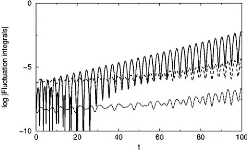
Figure 1 shows the logarithm of the three fluctuation in-tegrals

具

X₁2

典

,

具

X1X2

典

and

具

X2

2

_典

for the narrow resonance case. These are seen to be dominated by the exponential growth of

具

X₂2

典

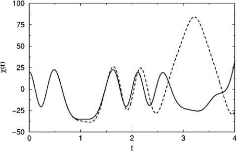
, while the other contributions grow more slowly. Therefore, the evolution is characterized by produc-tion of X2 particles. We now turn to the broad resonance regime, where things look quite different. Here, each of the fluctuation integrals grows rapidly as shown in Fig. 2. Sig-nificant mixing of the species occurs along with copious par-ticle production.

[image:8.612.315.558.56.209.2]

The behavior of the fluctuation integrals is consistent with the behavior of the time-dependent mixing angle ⌰. Here, the mixing plays a sub-dominant role in the narrow reso-nance regime 共Fig. 3兲with the mixing angle remaining near zero. This means that X₂ predominantly corresponds to the␹ field, such that the process is one of ␹ particle production, which is as expected. Concentrating on the time-dependent mixing angle in the broad resonance regime, Fig. 4, signifi-cant mixing between the fields is observed. The rapid varia-tion in the mixing angle indicates that mixing between the

FIG. 1. The logarithm of the fluctuation integrals具X1 2_典共

solid兲, 具X1X2典 共dashed兲, and 具X2

2_典

共dotted兲 for the narrow resonance re-gime.

FIG. 2. The logarithm of the fluctuation integrals具X1 2_典共

solid兲, 具X1X2典共dashed兲, and具X2

2_典

[image:8.612.53.294.58.206.2]

fields plays a very important role in the evolution of preheat-ing in the broad resonance regime. The large influence this has on the behavior of the system is clear from the evolution of the zero mode components␾(t) in Fig. 5 and␹(t) in Fig. 6.

B. Supersymmetric hybrid inflation

We now consider a hybrid inflationary model where the finite coupling of two fields plays an interesting role in the termination of slow roll inflation 关3兴. The particular model we study is based on softly broken supersymmetry关19兴with the potential

V共␴,N兲⫽1 2m␴

2_␴2_⫹1 4␬s

2_共N2_⫺2␴c2_兲2_⫹␬ s 2_N2_␴2_.

共3.1兲

The field ␴ plays the role of an inflaton during inflation while the field N is trapped in a false vacuum

具

N

典⫽

0. The inflaton rolls down the potential along the ␴ direction to reach a critical value ␴⫽␴c. Once ␴ reaches its critical value, the effective squared mass for the N field becomes negative and consequently it rolls down from the false vacuum to its global minimum through the mechanism of

spinodal instability 关11,12兴. Thus, inflation comes to an end and both the fields begin oscillations around their respective minima given by

␴⫽0, N⫽

冑

2␴_c. 共3.2兲

This is the onset of the preheating stage, which has been discussed in the literature关22,19,23兴. The difference between the supersymmetric hybrid potential and non-supersymmetric hybrid potentials lies in different coupling constants. In Eq.共3.1兲, there is only the single coupling pa-rameter ␬s, while in the non-supersymmetric version there can be at least two different coupling constants. The above potential, except for the ␴ mass term, can be derived very easily from the superpotential for F-term spontaneously su-persymmetry breaking:

W⫽␬s 2 ␴共N

2_⫺␴ c

2_{兲. 共3.3兲}

[image:9.612.320.560.55.208.2]

The appearance of a mass term for␴ in Eq. 共3.1兲 is due to the presence of soft supersymmetry breaking. Its presence is essential for slow roll inflation to produce adequate density perturbations and also to provide a correct tilt in the power

FIG. 3. Time-dependent mixing angle⌰(t) for the narrow reso-nance regime.

[image:9.612.54.298.58.201.2]

FIG. 4. Time-dependent mixing angle⌰(t) for the broad reso-nance regime.

FIG. 5. Zero mode evolution with fluctuation 共solid line兲 and without fluctuation 共dotted line兲 for␾(t) for the broad resonance regime.

[image:9.612.318.559.543.696.2] [image:9.612.54.294.562.708.2]

spectrum关19兴. The height of the potential during inflation is given by ␬s2␴c

4

. Similar potentials to Eq. 共3.1兲 can also be derived from D-term supersymmetry breaking as discussed in Refs. 关24兴. In these models the critical value ␴c and the height of the potential energy are related to the Fayet-Illipoulus term coming from an anomalous U共1兲 symmetry. As in any inflationary model, hybrid inflation is constrained by the Cosmic Background Explorer共COBE兲 关25兴. This im-poses the bound

␬s␴c⬇1.27⫻1015兩␩兩 GeV, 共3.4兲 where␩ is one of the slow roll parameters which determines the slope of the power spectral index 关25兴. For our purpose we fix it to be兩␩兩⬃0.01.

In order to discuss the details of the physics we mention here the equivalence between Eq. 共3.1兲 and Eq. 共2.2兲. This helps us to establish direct relationship with our earlier analysis:

␾⬅␴, ␹⬅N, ␦␾⬅␦␴, ␦␹⬅␦N,

␭⫽0, ␬⬅6␬s2, g⬅2␬s, m_␾⬅m_␴,

m_␹2⬅⫺2␬s2␴_c2. 共3.5兲 Notice that m_␹2 is negative. An interesting feature of the hy-brid model is that irrespective of the values of the parameters ␬s, ␴c, and m␴, as long as they satisfy the COBE con-straints, the behavior of the mean fields follow a common pattern once they begin to oscillate关19兴. First of all, the mass term for the␴ field, m_␴, becomes less dominant compared to the effective frequency for the two fields, which is given by the effective mass for the two fields during oscillations

meff␴⫽meffN⫽2␬s␴cⰇm␴. 共3.6兲 Hence, there is a single natural frequency of oscillation, thanks to supersymmetry. Since the masses of the fields are the same at the global minima, there exists a particular solu-tion of the equasolu-tions of mosolu-tion for the␴ and N fields. Their trajectory follows a straight line towards their global minima:

N⫽⫾

冑

2共␴c⫺␴兲. 共3.7兲 The maximum amplitude attained by the␴ field is⬃␴c, while the other field attains a larger amplitude N⫽

冑

2␴c. 共We remind readers that ␴⫽␴_c corresponds to the point where the effective mass for N field changes its sign.兲This is the point of instability which we need to discuss here. From Eq.共3.1兲we notice that prior to the oscillations of the fields, and during the oscillations, the effective mass square for␴ is always positive. However, this is not the case for N, and its mass square can be positive as well as negative even during the oscillations of the fields, provided the amplitudes are large enough. If the amplitudes for ␴ and N are such that they satisfy Eq.共3.7兲, then the effective mass square for the N field is in fact always negative for ␴⬍␴c. If the ampli-tudes are large enough such that after the second order phase

transition the initial amplitude for ␴⬇␴c, it is then quite possible that near the critical point the effective mass for the field N vanishes completely. As far as the motion of the mean field without including fluctuations is concerned this does not provide any new insight. However, if the fields are quan-tized then the perturbations in the field, especially for ␦N, grow exponentially because␻_N2 in Eq.共2.26兲becomes nega-tive for sufficiently small momentum k. This shows that the vacuum is unstable near the critical point␴c.

Another intuitive way to appreciate this point is to con-sider the adiabatic condition for the vacuum. The adiabatic evolution for the zero mode evolution for N field is given by

兩␻˙ N兩Ⰶ␻N

2

. This condition is maximally violated at the point where the effective mass square for N becomes zero, and, violation in adiabatic evolution of the zero mode for N sug-gests that many fluctuations of ␦N are produced during the finite period when the adiabaticity is broken 关23兴. This ex-planation is quite naive because the overall production of particles and fluctuations depends also upon the global be-havior of the zero mode fields. The effect of corrections due to fluctuations might affect the production of particles and this is the point we are going to emphasize in our numerical simulations.

In some sense the hybrid model is quite different from chaotic inflationary models. In chaotic models, the inflaton field rolls down with an amplitude ⬃1/(mt), where m is the mass of the oscillating field. However, in the hybrid model the amplitude of the oscillations die down very slowly, al-lowing many oscillations of the␴and N fields in one Hubble time. Thus, one could expect large amplitude oscillations of the fields for a long time. This crucially depends on the pa-rameter␴c. If␴cⰆMp, then we notice that effective masses for ␴ and N fields during oscillations are much larger than the Hubble parameter. The Hubble parameter is given by H ⬇␬␴c2_{/ M}

pduring inflation, so,

meff␴

H ⫽ meffN

H ⬇ Mp

␴cⰇ1, 共3.8兲

provided the scale of ␴c is quite small compared to the Planck mass, we can effectively neglect the expansion of the Universe.

In the supersymmetric hybrid model there are two re-gimes of interest. Just after the mass square of the N field becomes negative, the fields begin to oscillate with an am-plitude which decreases as⬀1/t2. When the field amplitude drops below兩N(t)/

冑

2␴c⫺1兩⭐1/3, the amplitude of the os-cillations decreases as⬀1/t. In this regime, when the expan-sion of the Universe is neglected, the amplitude of the oscil-lations remains constant and the osciloscil-lations are harmonic:

N共t兲

冑

2␴c⬇1⫹

1

3cos共meff␴t兲. 共3.9兲

In this paper we are neglecting the expansion of the Uni-verse. We concentrate upon two regimes–one with large am-plitude oscillations which leads to the following parameters:

␭⫽0, ␬⫽24, g⫽4, m_␴2⫽0,

m_N2⫽⫺16⫻10⫺12,

␴共0兲⫽1.4⫻10⫺6,

N共0兲⫽1⫻10⫺15, 共3.10兲 and the other with small amplitude oscillations with the pa-rameters

␭⫽0, ␬⫽24⫻10⫺6, g⫽4⫻10⫺3,

m_␴2⫽0, mN 2_⫽⫺

4⫻10⫺12,

␴共0兲⫽0.24⫻10⫺3, N共0兲⫽0.66⫻10⫺3.

共3.11兲 The coupling constants are dimensionless while the other dimensionful parameters are denoted in Planck units. We find below a marked difference in the zero mode behavior of the fields␴ and N in these two cases, depending on whether the fluctuations are taken into account or neglected.

In parameter set共3.10兲, we study the features of the fields with a large amplitude. This can happen when the ␴ and N fields begin their oscillations just after the end of inflation. As mentioned earlier, after the end of inflation the maximum amplitude attained by the mean fields can be quite large ␴

⫽␴c, and N⫽

冑

2␴c. This is precisely the initial condition we have chosen for the mean fields for our numerics, as shown in Fig. 7. The values for ␬s and␴ccan be evaluated from Eq. 共3.5兲, which yields

␬s⫽2, ␴c⫽

冑

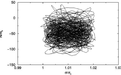
2⫻10⫺6. 共3.12兲 We notice that the evolution for ␴ and N fields without taking into account the fluctuations are anharmonic, see Fig. 7, and, their trajectories in the␴-N plane is a straight line, as shown in Fig. 8. However, switching on the fluctuations leads to a completely chaotic trajectory as shown in Fig. 9. The departure from the straight line trajectory is quite

sig-nificant and it tells us that the renormalized zero mode equa-tions have different contribuequa-tions to the parameter 6␬s2 and to the effective mass of the N field. This mismatch in the frequencies of the zero mode equations for␴ and N leads to an irregular trajectory.

The other way to interpret this behavior is to think in terms of different effective mass corrections to ␴ and N fields, such that the effective frequencies of the oscillations for ␴ and N do not match each other at the bottom of the potential. This is certainly a nontrivial result. Nonetheless, the result is quite expected from the fact that the amplitude of the oscillations are quite large and the effective mass for the N field is zero at each and every oscillation when ␴

⫽␴c.

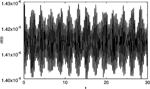
As we mentioned earlier, the frequencies of the oscilla-tions of the zero modes are different, as can be noticed in Figs. 10 and 11. The zero mode of ␴ influenced by the fluc-tuations oscillates around its minimum ␴⫽0 with a more rapid frequency than when fluctuations are neglected. This suggests that the effective mass correction to the zero mode for ␴ is coming solely from the finite coupling contribution from the N field. 共Note that we have already set the bare mass for m_␴⫽0.兲 The oscillations maintain the regularity with increasing and decreasing amplitude. However, the story is not the same for the zero mode behavior for the N field. The amplitude of N increases gradually and the

[image:11.612.54.296.58.201.2]

fre-FIG. 7. Evolution of␴ 共solid line兲and N共dotted line兲without fluctuations for parameter set共3.10兲.

FIG. 8. Trajectory for the fields␴and N for parameter set共3.10兲 without fluctuations.

[image:11.612.89.277.289.363.2] [image:11.612.319.556.559.707.2]

quency of the oscillations varies. We mention here that the effective mass for the N field can vanish at a critical point. As a result, the adiabatic condition for the N field is violated at those instants and this is the reason why the amplitude of the N field is enhanced rather than suppressed.

The evolution of the energy density is shown in Fig. 12. At first instance it seems quite odd that the energy density of the fluctuations does not increase further. One would naively expect a larger contribution of the energy density of␦␴ and ␦N. This is not the case here. The energy density for the mean fields and the fluctuations are equally shared. The rea-son is the correction due to the fluctuations. These correc-tions modify the effective mass of the N field and induce corrections to the coupling constants, namely ␬ and g. The coupling constants are modified in such a way that the tra-jectory of zero mode fields become irregular. Usually the production of fluctuations is not efficient in this case. This is quite similar to the situation of preheating in non-supersymmetric hybrid models关22兴. Even though we started with a supersymmetric hybrid model where at the bottom of the potential there is a single effective frequency, the situa-tion changes completely if the fluctuasitua-tions are taken into account. Essentially the coupling constants get a large cor-rection which does not preserve an effective single coupling constant for the evolution of the zero mode fields. This is precisely the reason why the zero mode trajectory becomes

irregular and also why the production of ␦␾ and ␦N is so low.

As a next example of the supersymmetric hybrid model we choose parameter set共3.11兲, with a small coupling␬sand small ␴c

␬s⫽2⫻10⫺3, ␴c⫽0.707⫻10⫺3. 共3.13兲

In this example, the coupling between the fields is quite small; g⫽4⫻10⫺3, and also the initial conditions for␴ and N have been chosen such that the fields oscillate around their respective minima. The maximum amplitude for ␴(0)

⫽␴c/3 and N(0)⫽(2

冑

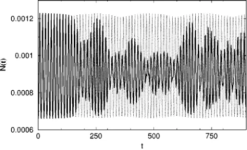
2/3)␴c is much below the critical point␴c. We remind the readers that the chosen initial con-ditions for the oscillations do not come naturally just after the end of inflation, therefore this example does not represent a real situation. In spite of this we study the particular situ-ation in order to notice the contrast in the behavior of the zero modes and the energy densities in the fluctuations. This particular set of initial conditions for ␴(0),N(0) offers an alternative example where spinodal instability in the N field does not take place. As a result the effective mass square for the N field never crosses zero and the adiabatic condition for the N field is not strongly broken. The oscillations of the mean fields ␴ and N are harmonic in nature, as shown in Figs. 13 and 14 by the dotted lines. The amplitudes are con-stant with a frequency given by Eq.共3.6兲. The oscillations of the mean fields is governed by Eqs. 共3.7兲 and 共3.9兲. The trajectory in the ␴-N plane is a straight line whose slope is governed by Eq.共3.7兲.

[image:12.612.319.560.56.204.2]

The effect of the fluctuations is also quite expected in this case. The amplitudes of the zero mode for ␴ and N fields decreases after a while and, in contrast to the preceding ex-ample, the frequency of the oscillations do not change very dramatically; see the behavior of zero mode in solid lines in Figs. 13 and 14. The trajectories for the zero mode evolution remain a straight line in this case, as shown in Fig. 15. This is quite reasonable for the parameters we have chosen, but an important observation is that the effect of fluctuations does not alter the straight line trajectory for the zero mode fields. This suggests that for small amplitude oscillations the cor-rections to the coupling constants,⌬␬ and⌬g, are such that

FIG. 10. Zero mode evolution for ␴(t) with fluctuations for parameter set共3.10兲.

FIG. 11. Zero mode evolution for N(t) with fluctuations for parameter set共3.10兲.

FIG. 12. Energy density stored in ␦␴ and ␦N fluctuations

[image:12.612.55.295.58.201.2]

the zero mode equations still have a similar oscillating fre-quency. This can be seen in Figs. 13 and 14. The production of ␦␴ and ␦N is not very significant because the energy density stored in␦␴and␦N does not grow rapidly. Thus the energy transfer from the zero modes to the fluctuation modes is not favorable for such small amplitude oscillations as can be seen in Fig. 16.

We conclude this section by mentioning that preheating in this supersymmetric hybrid model is quite interesting. De-pending on the amplitude of the oscillations of the fields, the behavior of the zero mode can be quite different. As a new feature we noticed that if the amplitude of the oscillations is close to the critical value ␴c, the effective mass square for the N field becomes negative and as a result the fluctuations of the field grows exponentially. However, the effect of fluc-tuations alters the coupling constants in such a way that the trajectory of the zero modes become irregular. Even though the adiabatic conditions seem to be broken for the N field near the critical value, the energy density transferred from the zero mode to the fluctuations is not sufficient. Our study reveals some interesting messages which we briefly mention here. We emphasize the point that the departure from the straight line trajectory of the zero mode is an essential fea-ture of a supersymmetric hybrid model if the fluctuations are taken into account. Even though, we have not included the

Hubble expansion, the results we have obtained are quite robust because supersymmetric hybrid inflationary models have a unique behavior of the fields which allows a smaller inflationary scale compared to the effective masses of the fields around their global minima. This suggests that during the oscillations, the expansion is felt much later, on a time scale determined by the parameters. This behavior is not shared by models where inflation is governed by a single field as in chaotic inflationary models. This undermines the production of quanta from the vacuum fluctuations. In sev-eral ways this affects the post inflationary radiation era of the Universe. Supersymmetric, weakly interacting dark matter formation and generation of baryonic asymmetry in the Uni-verse during preheating are the two most important frontiers which due to our results may warrant a careful revaluation.

[image:13.612.316.561.55.209.2]

In order to substantiate our claim that a due consideration of fluctuations after the end of inflation is an important fea-ture of any supersymmetric hybrid model, we have chosen an unphysical example which serves the purpose of making a vivid distinction. We stress here that the spinodal instability which is actually responsible for producing an irregular tra-jectory of the zero mode of the fields in a phase space is completely lacking if the amplitudes of the oscillations for ␴,N are small compared to the critical value␴c. This acts as

FIG. 13. Zero mode evolution for␴(t) with fluctuations共solid lines兲 and the without fluctuations 共dotted line兲 for parameter set

共3.11兲.

[image:13.612.55.295.57.208.2]

FIG. 14. Zero mode evolution for␹(t) with fluctuations共solid lines兲and without fluctuations共dotted line兲for parameter set共3.11兲.

FIG. 15. Zero mode trajectories with fluctuations for parameter set共3.11兲.

[image:13.612.320.560.540.686.2] [image:13.612.54.295.561.708.2]

a comparative study and shows that after the end of inflation, in a supersymmetric hybrid inflationary model, due to the spinodal instability in a field, a proper renormalization of the masses and the coupling constant have to be taken into ac-count.

IV. CONCLUSION

We have introduced a formalism to address the dynamics of N nonequilibrium, coupled, time varying scalar fields. We have shown that the one-loop corrections to the mean field evolution can be renormalized by dimensional regularization. For the sake of clarity and simplicity we restricted ourselves to Minkowski spacetime while deriving the renormalized equations of motion and the energy density of the system. We applied our formalism to a two-field case where we study the behavior of the quantized mode functions and the effect of fluctuations on the zero mode equations of motion for various parameters, including small and large amplitude os-cillations and large and weak coupling between two scalar fields. The varied couplings and amplitudes illustrate various facets of the intertwined dynamics of the two-fields which lead to a deeper understanding of the production of self-quanta and the transfer of energy density between the fields in a cosmological context.

As a special example we have chosen a two-field infla-tionary model which is genuinely motivated by supersymme-try and thus preserves the effective masses of the fields to be the same in their local minima. The model, as a paradigm, predicts inflation which comes to an end via a smooth phase transition, and the robustness of the model is confirmed by a slightly tilted spectrum of scalar density fluctuations within the COBE limit. The model parameters can be adjusted to give an inflationary scale covering a wide range of energy

scales from TeV to 1015 GeV. The phase transition leads to a spinodal instability in one of the fields which leads to co-herent oscillations of the fields around their global minima. The instability occurs in one of the fields which demands careful study of the back reaction to an otherwise growing mean field in an intertwined coupled bosonic system. An account of influence of the fluctuations gives rise to uneven contribution to the renormalized masses of the fields. This results in an irregular trajectory of the zero mode in a phase space, which breaks the coherent oscillations of the two fields. This prohibits an excessive production of particles from the vacuum fluctuations. This requires a careful re-evaluation of the successes of the production of weakly in-teracting massive particles and baryogenesis via out of equi-librium decay in supersymmetric hybrid inflationary models. Our study implies that exciting higher spin particles from the vacuum fluctuations of the coherent oscillations of the fields in a supersymmetric hybrid inflationary model demands careful reconsideration.

Even though we have neglected the effect of expansion in our calculation, our results are robust enough to claim that the fluctuations in a supersymmetric hybrid model do not grow if the back reaction of the fluctuations is taken into account in the mean field evolution. An extension of our formalism to an expanding universe deserves separate atten-tion.

ACKNOWLEDGMENTS

The authors are thankful to Mar Bastero-Gil and Michael G. Schmidt for helpful discussion. We thank Salman Habib for helpful comments on the manuscript. A.M. is partially supported by The Early Universe Network HPRN-CT-2000-00152.

关1兴A. Guth, Phys. Rev. D 23, 347共1981兲; E. W. Kolb and M. S.

Turner, The Early Universe共Addison-Wesley, Redwood City,

1990兲.

关2兴M. Kamionkowski and A. Kosowsky, Annu. Rev. Nucl. Part.

Sci. 49, 77共1999兲.

关3兴A. Linde, Phys. Lett. 129B, 177 共1990兲; E.J. Copeland, A.R. Liddle, D.H. Lyth, E.D. Stewart, and D. Wands, Phys. Rev. D 49, 6410共1994兲.

关4兴A. Albrecht, P.J. Steinhardt, M.S. Turner, and F. Wilczek, Phys.

Rev. Lett. 48, 1437 共1982兲; A.D. Dolgov and A.D. Linde,

Phys. Lett. B 116, 329共1982兲; L.F. Abbott, E. Farhi, and M.

Wise, ibid. 117, 29共1982兲.

关5兴D. Boyanovsky, H.J. De Vega, R. Holman, D.S. Lee, and A.

Singh, Phys. Rev. D 51, 4419共1995兲.

关6兴J. Traschen and R. Brandenberger, Phys. Rev. D 42, 2491

共1990兲; Y. Shtanov, J. Traschen, and R. Brandenberger, ibid.

51, 5438共1995兲.

关7兴L. Kofman, A. Linde and A. Starobinsky, Phys. Rev. Lett. 73,

3195共1994兲; Phys. Rev. D 56, 3258共1997兲; D. Boyanovsky,

M. D’Attanasio, H.J. de Vega, R. Holman, and D.-S. Lee, ibid. 52, 6805共1995兲; D. Boyanovsky, D. Cormier, H.J. de Vega, R.

Holman, A. Singh, and M. Srednicki, ibid. 56, 1939共1997兲.

关8兴Examples of reheating involving higher spin fields are

in-cluded in J. Baacke, K. Heitmann, and C. Pa¨tzold, Phys. Rev.

D 58, 125013 共1998兲; A.L. Maroto and A. Mazumdar, Phys.

Rev. Lett. 84, 1655共2000兲.

关9兴T. Prokopec and T.G. Roos, Phys. Rev. D 55, 3768共1997兲.

关10兴H.P. Nilles, M. Peloso, and L. Sorbo, J. High Energy Phys. 04, 4共2001兲.

关11兴D. Boyanovsky and H.J. de Vega, Phys. Rev. D 47, 2343

共1993兲.

关12兴D. Boyanovsky, D. Cormier, H.J. de Vega, R. Holman, and P.

Kumar, Phys. Rev. D 57, 2166 共1998兲; D. Cormier and R.

Holman, ibid. 60, 041301 共1999兲; 62, 023520 共2000兲; Phys.

Rev. Lett. 84, 5936共2000兲.

关13兴F. Cooper, S. Habib, Y. Kluger, E. Mottola, J.P. Paz, and P.R.

Anderson, Phys. Rev. D 50, 2848共1994兲.

关14兴F. Cooper, S. Habib, Y. Kluger, and E. Mottola, Phys. Rev. D

55, 6471 共1997兲; D. Boyanovsky, H.J. de Vega, R. Holman,

and J. Salgado, ibid. 59, 125009 共1999兲; J. Baacke and K.

Heitmann, ibid. 62, 105022共2000兲.

关15兴F. Cooper and E. Mottola, Phys. Rev. D 36, 3114共1987兲.

关16兴J. Baacke, K. Heitmann, and C. Pa¨tzold, Phys. Rev. D 55, 2320

关17兴J. Baacke, K. Heitmann, and C. Pa¨tzold, Phys. Rev. D 55, 7815

共1997兲.

关18兴J. Schwinger, J. Math. Phys. 2, 407共1961兲; L.V. Keldysh, Sov. Phys. JETP 20, 1018共1965兲.

关19兴M. Bastero-Gil, S.F. King, and J. Sanderson, Phys. Rev. D 60,

103517共1999兲.

关20兴R. Micha and M.G. Schmidt, Eur. Phys. J. C 14, 547共2000兲.

关21兴J. Baacke, K. Heitmann, and C. Pa¨tzold, Phys. Rev. D 56, 6556

共1997兲; 57, 6406共1998兲.

关22兴J. Garcia Bellido and A. Linde, Phys. Rev. D 57, 6075共1998兲.

关23兴G. Felder, J. Garcia-Bellido, P.B. Greene, L. Kofman, A. Linde and I. Tkachev, Phys. Rev. Lett. 87, 011601共2001兲.

关24兴E. Halyo, Phys. Lett. B 387, 43 共1996兲; P. Bine´truy and G. Dvali, ibid. 388, 241共1996兲; for earlier work on this subject see J.A. Casas and C. Mun˜oz, ibid. 216, 37共1989兲; J.A. Casas,

J. Moreno, C. Mun˜oz, and M. Quiros, Nucl. Phys. B328, 272

共1989兲.

关25兴E.F. Bunn, D. Scott and M. White, Astrophys. J. Lett. 441, L9