http://dx.doi.org/10.4236/ojs.2016.61015
A Comparison of Two Linear Discriminant
Analysis Methods That Use Block Monotone
Missing Training Data
Phil D. Young1, Dean M. Young2, Songthip T. Ounpraseuth3 1Department of Information Systems, Baylor University, Waco, TX, USA 2Department of Statistical Science, Baylor University, Waco, TX, USA
3Department of Biostatistics, University of Arkansas for Medical Sciences, Little Rock, AK, USA
Received 7 January 2016; accepted 23 February 2016; published 26 February 2016
Copyright © 2016 by authors and Scientific Research Publishing Inc.
This work is licensed under the Creative Commons Attribution International License (CC BY). http://creativecommons.org/licenses/by/4.0/
Abstract
We revisit a comparison of two discriminant analysis procedures, namely the linear combination classifier of Chung and Han (2000) and the maximum likelihood estimation substitution classifier for the problem of classifying unlabeled multivariate normal observations with equal covariance matrices into one of two classes. Both classes have matching block monotone missing training data. Here, we demonstrate that for intra-class covariance structures with at least small correlation among the variables with missing data and the variables without block missing data, the maxi-mum likelihood estimation substitution classifier outperforms the Chung and Han (2000) classifi-er regardless of the pclassifi-ercent of missing obsclassifi-ervations. Specifically, we examine the diffclassifi-erences in the estimated expected error rates for these classifiers using a Monte Carlo simulation, and we compare the two classifiers using two real data sets with monotone missing data via parametric bootstrap simulations. Our results contradict the conclusions of Chung and Han (2000) that their linear combination classifier is superior to the MLE classifier for block monotone missing multiva-riate normal data.
Keywords
Linear Discriminant Analysis, Monte Carlo Simulation, Maximum Likelihood Estimator, Expected Error Rate, Conditional Error Rate
1. Introduction
multivariate normally distributed populations Πi:Np
(
µi,Σ)
, i=1, 2, when monotone missing training data are present, where µi and Σ are theth
i population mean vector and common covariance matrix, respec- tively. Here, we re-compare two linear classification procedures for block monotone missing (BMM) training data: one classifier is from [1], and the other classifier employs the maximum likelihood estimator (MLE).
Monotone missing data occur for an observation vector xj when, if xji is missing, then xjk is missing
for all k>i. The authors [1] claim that their “linear combination classification procedure is better than the substitution methods (MLE) as the proportion of missing observations gets larger” when block monotone missing data are present in the training data. Specifically, [1] has performed a Monte Carlo simulation and has concluded that their classifier performs better in terms of the expected error rate (EER) than the MLE sub- stitution (MLES) classifier formulated by [2] as the proportion of missing observations increases. However, we demonstrate that for intra-class covariance training data with at least small correlations among the variables, the
MLES classifier can significantly outperform the classifier from [1], which we refer to as the C-H classifier, in terms of their respective EERs. This phenomenon occurs regardless of the proportion of the variables missing in each observation with missing data (POMD) in the training data set.
Throughout the remainder of the paper, we use the notation m n× to represent the matrix space of all m n×
matrices over the real field . Also, we let the symbol >n represent the cone of all n n× positive definite
matrices in n n× . Moreover, A′∈n m× represents the transpose of A∈m n× .
The author [3] has considered the problem of missing values in discriminant analysis where the dimension and the training-sample sizes are very large. Additionally, [4] has examined the probability of correct classi- fication for several methods of handling data values that are missing at random and use the EER as the criterion to weigh the relative quality of supervised classification methods. Moreover, [5] has examined missing obser- vations in statistical discrimination for a variety of population covariance matrices. Also, [6] has applied re- cursive methods for handling incomplete data and has verified asymptotic properties for the recursive methods.
We have organized the remainder of the paper as follows. In Section 2, we describe the C-H classifier, and we describe the MLES linear discriminant procedure when the training data from both classes contain identical
BMM data patterns. In Section 3, we describe and report the result of Monte Carlo simulations that examine the differences in the estimated EERs of the C-H and MLES classifiers for various parameter configurations, training-sample sizes, and missing data sizes and summarize our simulation results graphically. In Section 4, we compare the C-H and MLES linear classifiers using a parametric bootstrap estimator of the EER difference (EERD) on two actual data sets. We summarize our results and conclude with some brief comments in Section 5.
2. Two Competing Classifiers for
BMM
Training Data
2.1. The C-H Classifier for Monotone Missing Data
Suppose we have two p×Ni training observation matrices in the form
1 2 ,
i i i
⋅
Y Y
Z (1)
where
[
1 :]
ii i i k n
′ ×
′ ′
= ∈
U Y Z (2) denotes the ni complete-observation submatrix, and Yi2∈k×(Ni−ni) is the partial observation submatrix
whose first k measurements are non-missing, where Ni >ni, for i=1, 2. We denote a complete data ob-
servation vector by ij i j1 : ij
′
′ ′
=
u y z , where yi j1 ∈k×1 and zij∈(p k− ×)1 such that
(
)
1 11 1221 22
~ , i , ,
i
Y
ij p i p
Z
N ≡N
u Σ Σ Σ
Σ Σ
µ µ
µ (3)
where µYi1∈k×1, µZi∈(p k− ×)1,
> 11∈k k×
Σ , Σ12∈k× −(p k), and ( ) ( )
> 22∈ p k− × −p k
Σ with
1, 2; 1, 2, , i
i= j= n . Also, random samples of sizes Ni−ni are taken from distributions of the form
(
i2,)
k Y yy
N µ Σ , where µYi2∈k×1 and
>
yy∈k k×
Σ .
criminant function (LDF) for the subset of complete data Ui, i=1, 2, given in (2), which is
(
)
1(
)
1 2 1 2
1
, 2
W ≡ − ′ − − +
u u u Su u u u
where
1 1 ni
i ij j i
n =
=
∑
u u and
(
)(
)
2 1 1 1 2 1 , 2 i nij i ij i i j
n n = =
′
= − −
+ −
∑∑
u
S u u u u
are the complete-data sample mean and complete-data sample covariance matrix, respectively. They also use Anderson’s LDF for the data
[
Yi1:Yi2]
, (4) 1, 2i= , with k features and N1+N2 training observations, which is
(
)
1(
)
1 2 1 2
1 2
W ≡ − ′ − − +
y y y Sy y y y
with
(
)
1 2
1
,
i i i i i i
i
n N n
N
= + −
y y y (5)
where
1 1 1 1 ni
i i j j i
n =
=
∑
y y (6) denotes the sample mean for the first ni observations and the first k features from Yi1 in (1),
2 2 1
1 i
i
N i i j
j n i i
N n = +
=
−
∑
y y
denotes the sample mean for the first k features of the latter Ni−ni observations from Yi2 in (1), and
(
)(
)
2 2
1 1 1 1 2
1 2
i
N
itj i itj i i t j
N N = = =
′
= − −
+ −
∑∑∑
y
S y y y y
is the pooled sample covariance matrix for the incomplete training data (4), where t=1, 2, represent the subsets of (1) with non-missing data and BMM data, respectively, for i=1, 2.
The authors [1] have proposed the linear combination statistic
(
1)
,c
W ≡cWu+ −c Wy (7)
where c∈
[ ]
0,1 . One classifies an unlabeled observation vector x∈p×1 into Π1 if 0c
W ≥ (8)
and into Π2, otherwise. The conditional error rate (CER) for classifying an unlabeled vector x from Πi into j
Π using (8) is
( )
(
( )
)
( )
( )
2
1 2 1 2
2 2
1 0 | , , , , , ; ,
1 1
,
j
ij c c u y i
i i
i
CER W P W
f
−
− −
= − < ∈ Π
− ′ + −
= Φ
′
u u S y y S u y
h
h hΣ
µ (9)
, 1, 2
i j= , i≠ j, where
(
1)
with
(
)
1(
)
(
)
1(
)
1 2 1 2 1 2 1 2
1 1
and .
2 2
b≡ − u −u ′Su− u +u e≡ − y −y ′Sy− y + y
Also,
[
′ : ′]
′, =h r b (11) where r∈k×1 and b∈(p k− ×)1 , r≡ca1+ −
(
1 c)
d , b≡ca2 ,(
)
1 1 2 −
= y −
d S y y , 1
(
1 2)
−= u − =
a S u u
[
a1′ : a2′]
, with a1∈k×1, a2∈(p k− ×)1, and yi defined in (5). Thus, using (9) and assuming equal a prioriprobabilities, the CER for (8) is
( )
12( )
21( )
1
. 2
c c c
CER W = CER W +CER W (12)
If
1: 2: : : 1: 2 ,
≡ y u
θ y y S S u u
then, for (8), the EER of misclassifying an unlabeled observation vector x from Πi into Πj is
( )
( )
12( )
12 ,i i
i c ij
f
EER W E
− − − ′ + − = Φ ′ θ h h h Σ µ
, 1, 2
i j= , i≠ j. Thus, once again assuming equal a priori probabilities, the EER for (8) is
( )
12( )
21( )
1
. 2
c c c
EER W = EER W +EER W
In choosing c in (7), [1] have utilized the fact that the CER and EER will depend on the Mahalanobis distance for the complete and partial training observations and the corresponding training-sample sizes, Ni and ni,
1, 2
i= . Usually, when one has small CERs, at least one of the sample Mahalanobis distances
(
)
(
)
2 1
1 2 1 2 , , ,
Dw ≡ w −w ′Sw− w −w w=u y will be large. While ni and
2
Du determine the performance of Wu, the quantities Ni and
2
Dy dictate the performance of Wy. Hence, [1] have chosen c in relation to the training-sample sizes and the Mahalanobis dis- tances for the complete and incomplete training-data sets. Note that the implication for circumstances where
2 2
Du >Dy is that the information in the data-matrix component Zi, i=1, 2, in (1) contributes largely to the
discriminatory information. Hence, [1] uses
1 2 1 2 * 1 1 2 2
1 2 1 2
1 1
1 1 1 1
D
n n
c
D D
n n N N
− − − + = + + + u u y
to determine the linear combination classification statistic (7).
2.2. A Maximum Likelihood Substitution Classifier for Monotone Missing Training Data
The authors [7] have derived an MLE method for estimating parameters in a multivariate normal distribution with BMM data. The estimator of Σ in the [7] MLES classifier is a pooled estimator of the two individual
MLEs of Σ.
Below, we state the MLEs for two multivariate normal distributions having unequal means and a common covariance matrix with identical BMM-data patterns in both training samples.
Theorem. Let Πi be modeled by the multivariate normal densities Np
(
µi,Σ)
for i=1, 2, with1 2 i i i ≡ µ µ
and 11 12 21 22 . ≡ Σ Σ Σ
Σ Σ (14)
Also, let
(
)(
)
11, , 1 , i i NN i ij i ij i j=
′
≡
∑
− −A y y y y
(
)(
)
11, , 1 , i i nn i ij i ij i j=
′
≡
∑
− −A y y y y
(
)(
)
12, , 1 , i i nn i ij i ij i j=
′
≡
∑
− −A y y z z
and
(
)(
)
22, , 1 , i i nn i ij i ij i j=
′
≡
∑
− −A z z z z
where yij∈
[
Yi1:Yi2]
, and zij∈Zi with Yi1, Yi2, and Zi given in (1). Then, on the basis of two-step mono-tone training samples from populations Πi:Np
(
µi,Σ)
,i=1, 2, the MLEs of (13) and (14) are 1 11 122 21 22
ˆ ˆ
ˆ
ˆ
ˆ and ,
ˆ ˆ ˆ i i i ≡ ≡ Σ Σ Σ Σ Σ µ µ
µ (15)
respectively, where 2 11, , 1 11 2 1
ˆ i N ii ,
i i N = = ≡
∑
∑
A Σ 1 2 2 2 12 2 11, , 11, , 12, ,1 1 1
1 1
ˆ ,
i i i
N i n i n i
i i i
i i N − = = = = ≡
∑
∑
∑
∑
A A AΣ (16)
and
1
2 2 2
22 2 22 1, , 2 21, , 11, ,
1 1 1
1 1
1
2 2 2
11, , 11, , 12, ,
1 1 1
1 1
ˆ
,
i i i
i i i
n i n i n i
i i i
i i
i i
N i n i n i
i i i
n N − ⋅ = = = = = − = = = ≡ + ×
∑
∑
∑
∑
∑
∑
∑
∑
A A A
A A A
Σ
(17)
with µˆi1= yi, where yi is defined in (5),
(
)
1
2 ˆ ˆ12 22 1 2
ˆi i i i ,
−
≡ −z Σ Σ y −y
µ 1 1 , i n i ij j i n = ≡
∑
z z and 1 2 2 2 2 222 1, , 22, , 21, , 11, , 12, , 1 1 1 1 1
,
i i i i i
n i n i n i n i n i
i i i i i
− ⋅ = = = = = ≡ −
where yi1, yi2, Σˆ12, and Σˆ22, are defined in (5), (6), (16), and (17), respectively, for i=1, 2.
Proof: A proof is alluded to in [8]. The MLES classification statistic is
(
)
1(
)
2 1 2 1
1 ˆ
ˆ ˆ ˆ ˆ ,
2
MLE
W ≡ − ′ − − +
x
Σ
µ µ µ µ (18)
where µˆ1, µˆ2, and Σˆ are the MLEs defined in (15), and x∈p×1 is an unlabeled observation vector belonging to either Π1 or Π2. We classify the unlabeled observation vector x∈p×1 into Π1 if
0
MLE
W ≤ (19)
and into Π2, otherwise. Given that x∈ Π1, conditioning on ˆµij, i j, =1, 2, and Σˆ, and using the fact that
(
)
(
)
1 1 1 1
ˆ ˆ ~N 0,ˆ ˆ ˆ ˆ ,
δ′ − − δ′ − −δ
x
Σ µ Σ ΣΣ
where δˆ≡µ µˆ1− ˆ2, along with (15), (18), and (19), we have that
(
)
( )
12 ˆ1,ˆ2,ˆ MLE 0 | ˆ1,ˆ2, ;ˆ 1 1 1 ,
CER µ µ Σ ≡P W > µ µ Σ x∈ Π = − Φ w
where
(
)
1 2 1 1 1
2 1 1
ˆ ˆ ˆ ˆ ˆ ˆ ˆ ˆ ,
2
i i
w ≡δ′ − −δ− δ′ − + −µ
Σ ΣΣ Σ µ µ (20)
1, 2
i= . Similarly, given x∈ Π2,
(
)
( )
21 ˆ1, ˆ2,ˆ MLE 0 | ˆ1,ˆ2, ;ˆ 2 2 ,
CER µ µ Σ ≡P W ≤ µ µ Σ x∈ Π = Φ w
where w2 is given in (20). Thus, assuming equal a priori probabilities of belonging to Πi, i=1, 2, for an
unlabeled observation, we have
(
1 2)
( )
1( )
21 ˆ
ˆ,ˆ , 1 .
2
CER µ µ Σ ≡ − Φ w + Φ w (21)
Hence, the overall expected error rate is
(
1 2)
(
( )
1)
(
( )
2)
1 ˆ
ˆ,ˆ , 1 .
2
EER µ µ Σ ≡ −Eθ Φ w +Eθ Φ w
3. Monte Carlo Simulations
The authors [1] claim that “it can be shown that the linear combination classification statistic is invariant under nonsingular linear transformations when the data contain missing observations” and assume this invariance is also true for the MLES classifier. While their assertion might be true for the C-H classifier, it is not necessarily true for the MLE classifier. Because [1] do not consider covariance structures with moderate to high correlation, their results are biased toward the C-H classifier. Here, we show that the MLES classifier can considerably outperform the C-H classifier, depending on the degree of correlation among the variables with missing data and the variables without missing data.
Next, we present a description and results of a Monte Carlo simulation we have performed to evaluate the
EERD between the MLE and C-H classifiers for two multivariate normal configurations, Πi:Np
(
µi,Σ)
, 1, 2i= , using various training-sample sizes, dimensions, features with block missing data, differences in means, values of correlation among variables, and missing-data proportions. For the simulations, we define p to be the total number of feature dimensions and r to be the number of missing features so that r< p. Also, Ni denotes
the total training-sample size from population Πi, i=1, 2, and
(
1)
ρ ρ
≡ J+ − I
Σ
is the intraclass covariance matrix where ρ denotes the common population correlation among the features in the intraclass covariance matrix and J∈p p× denotes a matrix of ones.
command in PROC IML to generate 10,000 training-sample sets of size Ni, i=1, 2, for each parameter
configuration. Next, the MLE and C-H classifiers were computed, and their CERs were calculated for each training-sample set. Then, the differences between the CERs for the classifiers were averaged over the 10,000
CER differences for the two classifiers for each parameter configuration involving Ni, p, r, Σ, µi, and
POMD for the r features with monotone missing data, where i=1, 2. Thus, the EERD for the C-H and MLES
classifiers is
( )
(
)
1 2 1
1 ˆ
ˆ,ˆ , ,
K
j c j j
EERD CER W CER
K =
=
∑
− µ µ Σ where CER W
( )
c is defined in (12), CER(
µ µˆ1,ˆ2,Σˆ)
is given in (21), K is the total number of simulated training-data sets, and j denotes the jth simulated training-data set, where j∈{
1, 2,,K}
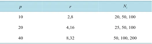
. We display the results of our two Monte Carlo simulations by graphing EERD against ρ =0.1, 0.3, 0.5, 0.7, 0.9 for various configurations of p, r, Ni, µ1, µ2, and POMD.The relationship between p and r was fixed at r=0.2p and r=0.8p. We chose these specific values of p
and r to evaluate EERD when the proportion of variables with missing data were both small and large relative to p. The choice of r and Ni depended on the value of p, and we provide the values of p, r, and Ni used in
the Monte Carlo simulation in Table 1. Lastly, we chose µ1∈p×1 such that
[
]
1 = 0, 0,, 0′
µ (22)
and µ2∈p×1 such that
2 dj, 0, 0, , 0,dj, 0, , 0 ,
′
=
µ (23)
with d1=0.5 and d2=3 to assess EERD for both small and large between-class separation. These values for µi, i=1, 2, given in (22) and (23), were chosen because they are similar to the population means used in
the simulation used in [1]. Furthermore, we contrasted (8) and (19) using POMD = 0.5, 0.8 for the r covariates with BMM data, and as in [1], we chose Ni> p to avoid singularity of the estimated covariance matrices. The
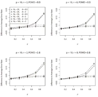
comparison criterion EERD is plotted against ρ for various combinations of p, r, dj, Ni, and POMD in
Figure 1 and Figure 2, i j, =1, 2. Although we simulated values for EERD for p=10, 20, 40, we omitted the graphs for p=20 because the graphs are similar to the plots for p=10 and p=40. The graphs for
20
p= can be obtained from the authors.
Figure 1, Figure 2 illustrate that the EERD is consistently positive for the values of p, r, Ni, ρ, dj, and
POMD examined here. Moreover, the figures indicate that the primary parameters that influence the dominance of the MLES classifier are ρ and dj, j=1, 2. For all feature dimensions considered here, the C-H and
MLES classifiers were competitive for ρ=0.1. More importantly, for ρ >0.1, EERD increased as ρ increased for all p, r, Ni, µ1, µ2, and POMD considered here. The most noteworthy increase in the EERD was for 0.7≤ ≤ρ 0.9 when d1=0.5, where EERD increased by approximately 0.10. This increase occurred for all specified values of p, r, Ni, and POMD, and, thus, supported the superiority of the MLES
classifier in terms of EERD for these configurations. Additionally, we noted that EERD≈0.20 when ρ=0.9, 1 0.5
d = , and other parameters are allowed to vary.
[image:7.595.186.449.641.718.2]The MLES classifier especially outperformed the C-H classifier when d1=0.5 for ρ>0, as compared to when d2=3. The smaller values of EERD for d2=3 can be attributed to the fact that for a relatively large
Table 1. Dimensions and sample sizes for the Monte Carlo simulation.
p r Ni
10 2,8 20, 50, 100
20 4,16 25, 50, 100
Figure 1. Graphs of the EERD versus ρ for fixed values of Ni, r, dj, POMD, and p = 10.
Mahalanobis distance when d2=3 and ρ =0.1, the EERs for both classifiers are small, thus yielding a smaller EERD.
As we used a large number of simulation iterations, we obtained max
{
s e EERD . .(
)
}
<0.003ξ , where ξ is
the grid of parameter vectors considered in the simulation. Thus, the relatively small estimated standard errors also support our claim that EERD>0 for ρ>0.1 for the parameter configurations considered here. As
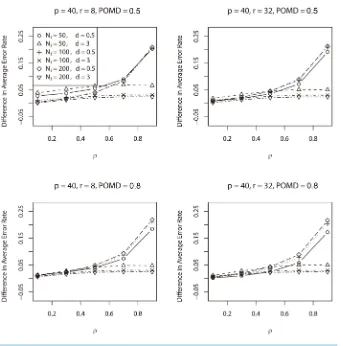
Figure 1, Figure 2 indicate, the contrasting values of p, r, Ni, and POMD contribute marginally, if at all, to
EERD. Regardless of the combination of parameter values considered here, the MLES classifier dominates the
C-H classifier in terms of EERD.
In summary, the simulation results indicated that the MLES classifier became increasingly superior to the C-H
classifier as the correlation magnitude among the features with no missing data and the features with BMM data increased.
We remark that the standard errors for the EERD in the [1] simulations are not sufficiently small enough to conclude a difference in the ERRs of the two competing classifiers. Hence, their claim that the C-H classifier outperforms the MLES classifier as the percent of missing observations increases is questionable.
Figure 2. Graphs of the EERD versus ρ for fixed values of Ni, r, dj, POMD, and p = 40.
4. Two Real-Data Examples
4.1. Bootstrap Expected Error Rate Estimators for the C-H and MLE Classifiers
In this section, we compare the parametric bootstrap estimated ERRs of the C-H and MLES classifiers for two real-data sets each having two approximate multivariate normal populations with different population means and equal covariance matrices. First, we define the bootstrap ERR estimator for the C-H classifier, EERBoot(C H- ). Let
1 ˆ
µ , µˆ2, and Σˆ be the MLEs of µ1, µ2, and Σ, respectively, defined in Theorem 1. Also, let * 1 ˆ
µ , µˆ*2, and
*
ˆ
Σ be the bootstrap estimates of µˆ1, µˆ2, and Σˆ, respectively, calculated using the parametric bootstrap training-sample data
* * 1 2 *
i i i
⋅
Y Y
Z (24)
that is generated from Np
( )
µˆ ,i Σˆ , i=1, 2. Then, conditioning on µˆ*i, i=1, 2, and Σˆ*, the bootstrap CERs for the C-H classifier are
( )
( )
2 *( )
2 * * ** * ˆ
1 1
ˆ
i i
i ij c
f CER W
− −
− ′ + −
≡ Φ
′
h h Σh
µ
for i j, =1, 2, i≠ j, where Wc*,
*
h , and f* are similar in definition to Wc, h, and f in (7), (11), and (10),
( )
( )
( )
* * * * * *
12 21
1
. 2
c c c
CER W ≡ CER W +CER W (25)
Also, conditioning on µˆi*, i=1, 2, and Σˆ*
, the bootstrap CERs for the MLES classifier are
(
)
( )
2* * * * * * * * 1 2 ˆ 1 2 ˆ
ˆ ,ˆ , 1 j 0 | ˆ ,ˆ , ; ,
ij MLE i
CER µ µ Σ ≡P − − W > µ µ Σ x∈ Π
where x is a complete unlabeled observation from Π1Π2, *
MLE
W is similar in definition to WMLE in (18),
and i j, =1, 2, i≠ j. Given x∈ Π1 and
* * * 1 2
ˆ ˆ ˆ
δ ≡µ −µ , we have
(
)
( )
* * * * * 12 ˆ1,ˆ2,ˆ 1 1 ,
CER µ µ Σ = − Φ w
and given x∈ Π2,
(
)
( )
* * * * * 21 ˆ1,ˆ2,ˆ 2 ,
CER µ µ Σ = Φ w
where
(
)
1 2
* * * 1 * 1 * * * 1 * * 2 1 1
ˆ ˆ ˆ ˆ ˆ ˆ ˆ ˆ ˆ ˆ , 1, 2.
2
i i
w δ δ δ i
−
− − −
′ ′
≡ + − =
Σ ΣΣ Σ µ µ µ
Thus, assuming equal a priori probabilities of belonging to Πi, i=1, 2, for an unlabeled observation, we
have
(
)
( ) ( )
* * * * * *
1 2 1 2
1 ˆ
ˆ ,ˆ , 1 .
2
CER µ µ Σ = − Φ w + Φ w (26)
Hence, the estimated parametric bootstrap EERD for the C-H and MLES classifiers is
Boot
(
Boot( - ) Boot( ))
11
,
K
j C H j MLE j
EERD CER CER
K =
≡
∑
− (27)where j denotes the jth simulated training-data set for j∈
{
1, 2,,K}
. We use (27) to compare the C-H andMLES classifiers for two real-data sets given in the following subsections.
4.2. A Comparison of the C-H and MLE Classifiers for UTA Admissions Data
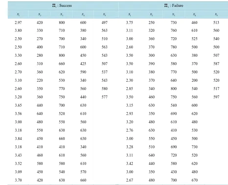
The first data set was supplied by the Admissions Office at the University of Texas at Arlington and imple- mented as an example in [1]. The two populations for the UTA data are the Success Group for the students who receive their master’s degrees (Π1) and the Failure Group for students who do not complete their master’s degrees (Π2). Each training sample is composed of ten foreign students and ten United States students. Each foreign student had 5 variables associated with him or her. The variables are X1 = undergraduate GPA, X2 = GRE verbal, X3 = GRE quantitative, X4 = GRE analytic, and X5 = TOEFL score. For each observation in both data sets, variables X1, X2, X3, and X4 are complete; however, X5 contains monotone missing data. The
UTA data set as seen in [1] can be seen in Table 2.
Also, the common estimated correlation matrix for the UTA data is
1.000 0.145 0.066 0.199 0.373 0.145 1.000 0.404 0.494 0.767 ˆ 0.066 0.404 1.000 0.129 0.493 .
0.199 0.494 0.129 1.000 0.392 0.373 0.767 0.493 0.392 1.000
UTA
−
−
= − − −
−
C (28)
We remark that only one sample correlation coefficient in the last column of (28) has a magnitude exceeding 0.50, which reflects relatively low correlation among the four features without BMM data with the one feature having BMM data.
Table 2. UTA Admissions office.
1
Π : Success Π2: Failure
1
x x2 x3 x4 x5 x1 x2 x3 x4 x5
2.97 420 800 600 497 3.75 250 730 460 513
3.80 330 710 380 563 3.11 320 760 610 560
2.50 270 700 340 510 3.00 360 720 525 540
2.50 400 710 600 563 2.60 370 780 500 500
3.30 280 800 450 543 3.50 300 630 380 507
2.60 310 660 425 507 3.50 390 580 370 587
2.70 360 620 590 537 3.10 380 770 500 520
3.10 220 530 340 543 2.30 370 640 200 520
2.60 350 770 560 580 2.85 340 800 540 517
3.20 360 750 440 577 3.50 460 750 560 597
3.65 440 700 630 3.15 630 540 600
3.56 640 520 610 2.93 350 690 620
3.00 480 550 560 3.20 480 610 480
3.18 550 630 630 2.76 630 410 530
3.84 450 660 630 3.00 550 450 500
3.18 410 410 340 3.28 510 690 730
3.43 460 610 560 3.11 640 720 520
3.52 580 580 610 3.42 440 580 620
3.09 450 540 570 3.00 350 430 480
3.70 420 630 660 2.67 480 700 670
and ni=10 for i=1, 2. Additionally, the parametric bootstrap multivariate normal distribution parameters, which are the MLEs for the multivariate normal population parameters given in Theorem 1, are
[
]
1
ˆ = 3.171, 409, 644, 526.25, 577.01′ µ
and
[
]
2
ˆ = 3.087, 430, 649, 519.75, 562.66′
μ
for the means of Π1 and Π2, respectively, with common covariance matrix
0.150 6.020 2.760 8.540 6.510
6.020 11504.500 4683 5859.375 3711.097 ˆ 2.760 4683 11701.500 1518.625 2406.740 .
8.540 5859.375 1518.625 12229.187 1953.163 6.510 3711.097 2406.740 1953.163 2034.414
−
−
= − − −
−
Σ
Subsequently, we obtained EERDBoot = −0.027 with
(
)
Boot. . 0.001
s e EERD = , which indicated that the C-H
classifier yielded slightly better discriminatory performance compared to the MLES classifier for the UTA data. The fact that the C-H procedure slightly outperformed the MLES classifier for the UTA data set in terms of
the C-H classifier does not require or use information in the correlation between the features with no missing data and the features with missing data. However, the MLES classifier does require at least a moderate degree of correlation between some features with no missing data and the feature with missing data to yield a more effective supervised classifier than the C-H classifier.
4.3. A Comparison of the C-H and MLE Classifiers on the Partial Iris Data
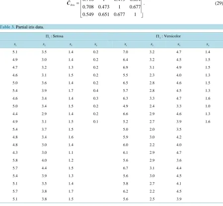
The second real-data set on which we compare the C-H and MLES classifiers is a subset of the well-known Iris data, which is one of the most popular data sets applied in pattern recognition literature and was first analyzed by R. A. Fisher (1936). The data used here is given in Table 3.
The University of Irvine Machine Learning Repository website provides the original data set, which contains 150 observations (50 in each class) with four variables: X1 = sepal length (cm), X2 = sepal width (cm), X3 = petal length (cm), and X4 = petal width (cm). This data set has three classes: Iris-setosa (Π1), Iris-versicolor (Π2), and Iris-virginica (Π3). We have used a subset of the original Iris data set by taking only the first 20 obser- vations from Π1 and Π2 and omitting the Iris-virginica group (Π3). We emphasize that the variables in the partial Iris data are much more highly correlated than the variables in the UTA data. The estimated correlation matrix is
1 0.716 0.708 0.549 0.716 1 0.473 0.651
ˆ .
0.708 0.473 1 0.677 0.549 0.651 0.677 1
Iris
=
C (29)
Table 3. Partial iris data.
1
Π : Setosa Π2: Versicolor
1
x x2 x3 x4 x1 x2 x3 x4
5.1 3.5 1.4 0.2 7.0 3.2 4.7 1.4
4.9 3.0 1.4 0.2 6.4 3.2 4.5 1.5
4.7 3.2 1.3 0.2 6.9 3.1 4.9 1.5
4.6 3.1 1.5 0.2 5.5 2.3 4.0 1.3
5.0 3.6 1.4 0.2 6.5 2.8 4.6 1.5
5.4 3.9 1.7 0.4 5.7 2.8 4.5 1.3
4.6 3.4 1.4 0.3 6.3 3.3 4.7 1.6
5.0 3.4 1.5 0.2 4.9 2.4 3.3 1.0
4.4 2.9 1.4 0.2 6.6 2.9 4.6 1.3
4.9 3.1 1.5 0.1 5.2 2.7 3.9 1.6
5.4 3.7 1.5 5.0 2.0 3.5
4.8 3.4 1.6 5.9 3.0 4.2
4.8 3.0 1.4 6.0 2.2 4.0
4.3 3.0 1.1 6.1 2.9 4.7
5.8 4.0 1.2 5.6 2.9 3.6
5.7 4.4 1.5 6.7 3.1 4.4
5.4 3.9 1.3 5.6 3.0 4.5
5.1 3.5 1.4 5.8 2.7 4.1
5.7 3.8 1.7 6.2 2.2 4.5
[image:12.595.88.538.307.722.2]In (29), all estimated correlation coefficients in the last column had a magnitude greater than 0.50, which reflects a moderate degree of correlation among the features X1, X2, and X3, and the feature X4, which has
BMM data.
For the Iris subset data, which can be found in Table 3, we used 10,000 bootstrap iterations, Ni =20, 10
i
n = , POMD=0.50, p=4, and r=1, where i=1, 2, for calculating EERDBoot. Hence, the overall proportion of missing observations for the Iris subset data is greater than that of the UTA data set. The bootstrap parameters corresponding to Π1 and Π2 are
[
]
1
ˆ = 5.035, 3.48,1.435, 0.235′ µ
and
[
]
2
ˆ = 5.975, 2.76, 4.255,1.325 ,′ µ
respectively, with common covariance matrix
0.273 0.147 0.124 0.045 0.147 0.154 0.062 0.040
ˆ .
0.124 0.062 0.111 0.035 0.045 0.040 0.035 0.024
=
Σ
For the parametric bootstrap estimate for EERD corresponding to the C-H and MLES classifiers applied to the subset of the Iris data set, we obtained EERDBoot =0.11 with s e EERD . .
(
Boot)
=0.001, which indicated that EER(MLE)EER(C H- ). Consequently, because of the relatively large correlations among the variables with no missing data, namely, X1, X2, X3, and the variable with missing data, X4, the MLES classifier convincingly outperforms the C-H classifier in terms of EERD. This evidence essentially contradicts the conclusion in [1] that the C-H classifier is superior to the MLES classifier when the proportion of observations with missing data is substantial, regardless of the covariance structure.5. Conclusions
In this paper, we have considered the problem of supervised classification using training data with identical
BMM data patterns for two multivariate normal classes with unequal means and equal covariance matrices. In doing so, we have used a Monte Carlo simulation to demonstrate that for the various parameter configurations considered here, ρ, not POMD, has the greatest impact on EERD. We have also concluded that the MLES
classifier outperforms the C-H classifier for all considered parameter configurations involving intra-class covariance structures when ρ≥0.1 and becomes an increasingly superior statistical classification procedure as
ρ approaches 1. This conclusion essentially contradicts the simulation results of [1].
We also have compared the MLE and C-H classifiers on two real training-data sets using EERDBoot in (27). From the real data set in [1], we have demonstrated that the C-H classifier can perform slightly better than the
MLES classifier. Moreover, we have used a subset of the prominent Iris data set from [9] to illustrate that when the magnitude of the correlation among features without missing data and features with missing data is moderate to large, the MLES classifier is superior to the C-H classifier.
References
[1] Chung, H.-C. and Han, C.-P. (2000) Discriminant Analysis When a Block of Observations Is Missing. Annals of the
Institute of Statistical Mathematics, 52, 544-556.
[2] Bohannon, T.R. and Smith, W.B. (1975) Classification Based on Incomplete Data Records. ASA Proceeding of Social
Statistics Section, 67, 214-218.
[3] Jackson, E.C. (1968) Missing Values in Linear Multiple Discriminant Analysis. Biometrics, 24, 835-844. http://dx.doi.org/10.2307/2528874
[4] Chang, L.S. and Dunn, O.J. (1972) The Treatment of Missing Values in Discriminant Analysis—1. The Sampling Ex-periment. Journal of the American Statistical Association, 67, 473-477.
Journal of the American Statistical Association, 71, 842-844. http://dx.doi.org/10.1080/01621459.1976.10480956 [6] Titterington, D.M. and Jian, J.-M. (1983) Recursive Estimation Procedures for Missing-Data Problems. Biometrika
Trust, 70, 613-624. http://dx.doi.org/10.1093/biomet/70.3.613
[7] Hocking, R.R. and Smith, W.B. (2000) Estimation of Parameters in the Multivariate Normal Distribution with Missing Observations. Journal of the American Statistical Association, No. 63, 159-173.
[8] Anderson, T.W. and Olkin, I. (1985) Maximum-Likelihood Estimation of the Parameters of a Multivariate Normal Distribution. Linear Algebra and Its Applications, 70, 147-171. http://dx.doi.org/10.1016/0024-3795(85)90049-7 [9] Fisher, R.A. (1936) The Use of Multiple Measurements in Taxonomic Problems. Annals Eugenics, 7, 179-188.