DETER M INING THE R A N G E OF
PR EDICTIO NS FOR CALIBRATED
A G EN T-BA SED SIM ULATION MODELS
By
D ongF ang S h i
,M S c
SUBMITTED FOR THE DEGREE OF DOCTOR OF PHILOSOPHY
AT
All rights reserved
INFORMATION TO ALL USERS
The qu ality of this repro d u ctio n is d e p e n d e n t upon the q u ality of the copy subm itted.
In the unlikely e v e n t that the a u th o r did not send a c o m p le te m anuscript and there are missing pages, these will be note d . Also, if m aterial had to be rem oved,
a n o te will in d ica te the deletion.
uest
ProQuest 11003739
Published by ProQuest LLC(2018). C op yrig ht of the Dissertation is held by the Author.
All rights reserved.
This work is protected against unauthorized copying under Title 17, United States C o d e M icroform Edition © ProQuest LLC.
ProQuest LLC.
789 East Eisenhower Parkway P.O. Box 1346
D E C L A R A T IO N
I declare th a t the work presented in this thesis is my own, except where
T able o f C o n ten ts iii
L ist o f T ables viii
L ist o f F igures x
A b stra c t xii
A ck n ow led gem en ts x iv
1 IN T R O D U C T IO N 1
1.1 INTRODUCTION ... 1
1.2 RESEARCH O B J E C T IV E S ... 4
1.2.1 Main O b je c tiv e ... 4
1.2.2 Secondary O b je c tiv e s... 5
1.3 BRIEF OVERVIEW OF A P P R O A C H ... 5
1.4 THESIS S T R U C T U R E ... 6
2 A G E N T -B A S E D S IM U L A T IO N 10 2.1 Introduction to the World of C o m p le x ity ... 11
2.1.1 W hat is C o m p lex ity ? ... 11
2.1.1.1 C o m p le x ity ... 11
2.1.1.2 Fingerprints of The C o m p l e x ... 12
2.1.2 Tipping Points ... 14
2.1.3 Why is Agent-based Simulation Suitable to Study CAS? . . . 16
2.2 Agent-based Simulation as a Young F ie l d ... 17
2.2.1 Multi-Agent Systems (M A S )... 17
2.2.2 W hat is an A g e n t ? ... 18
2.2.3 ABS Vs Traditionally S im u la tio n ... 22
2.2.4 Overview of ABS Application A re a s ... 26
2.2.4.1 Movement P a tte r n s ... 27
2.2.4.2 Economic Agent-based Models ... 29
2.2.4.3 Sociological Agent-based Models ... 30
2.2.4.4 Military Agent-based M o d e l s ... 31
2.3 Review of ABS T o o ls ... 32
2.3.1 Graphical Tools for ABS Model B u ild in g ... 32
2.3.2 Tools for A B S ... 33
2.3.2.1 Three ABS Tools Groups ... 34
2.3.2.2 A Brief List of ABS T o o l s ... 36
2.4 Summary ... 37
3 C A L IB R A T IO N OF A G E N T -B A S E D SIM U L A T IO N M O D ELS 38 3.1 REVIEW OF VERIFICATION & VALIDATION (V&V) OF ABS . . 39
3.1.1 Introduction to V & V ... 39
3.1.2 Principles of V&V ... 40
3.1.3 V&V T e c h n iq u e s ... 42
3.1.4 V&V for A B S ... 44
3.2 ABS MODEL P R E D IC T IO N ... 46
3.2.1 Difficulties In Using ABS For P r e d ic t io n ... 47
3.2.2 Inverse P ro b le m ... 48
3.2.3 Existing ABS Models Used For P red ictio n s... 49
3.2.3.1 Forecasting Hits in the J-pop (popular music in Japan) Market (Makoto, 2000)... 50
3.2.3.2 UK Pay-TV Subscriber Model (Twomey and Cadman, 2002) 52
3.2.3.3 D iscussion... 53
3.3 CALIBRATING M O D E L S ... 54
3.3.1 Markov Chain Monte Carlo (MCMC) Based Calibrating Method 54 3.3.1.1 A Brief Introduction To M C M C ... 54
3.3.1.2 Applying MCMC when Fitting Simulation Models . 55 3.3.1.3 Applications ... 56
3.3.1.4 Merits Of The M e th o d ... 58
3.3.1.5 Drawbacks Of The M e t h o d ... 59
3.3.2 Brooks et al. (1994) Method ... 59
3.3.3 Remarks On The Existing Model Calibrating Methods . . . . 61
3.4 S U M M A R Y ... 61
4 A G E N T -B A S E D M A R K E T IN G D IF F U S IO N M O D E L S 63 4.1 ABS FOR MARKETING ... 64
4.2 DIFFUSION M O D E L S ... 66
4.2.1 Bass (1969) Diffusion Model (BM) ... 67
4.2.2 Extensions to Bass (1969) Diffusion M o d e l ... 70
4.2.2.1 Generalized Bass Model (G B M )... 70
4.2.2.2 Successive G en eratio n s... 71
4.2.3 R e m a rk s... 71
4.2.3.1 M e r its ... 72
4.2.3.2 L im ita tio n s ... 72
Study (Kjima and Hirata, 2 0 0 4 ) ... 77
4.3.3 Remarks on the ABS Diffusion M o d e ls ... 79
4.3.3.1 Elements of ABS diffusion m o d els... 79
4.3.3.2 Limits of ABS diffusion m o d e l s ... 80
4.4 S U M M A R Y ... 81
5 R E S E A R C H M E T H O D O L O G Y 82 5.1 M E T H O D O L O G Y ... 82
5.1.1 A Flow Chart of The M e th o d o lo g y ... 83
5.2 CHOICE OF MODEL FOR THE RESEARCH ... 84
5.3 ADVANTAGES OF THE METHODOLOGY ... 84
5.4 DISADVANTAGES OF THE M E T H O D O L O G Y ... 85
5.5 DIFFERENCE IN THE METHODOLOGY TO THE PREVIOUS GROUND WATER S T U D Y ... 85
6 A G E N T -B A S E D C O N S U M E R M O D EL 87 6.1 MODEL O V E R V IE W ... 87
6.2 MODEL DESCRIPTION ... 89
6.2.1 Agents’ A t t r i b u t e s ... 90
6.2.2 Environment A t t r i b u t e s ... 92
6.2.3 Interactions in the M o del... 92
6.2.4 Rules on C o n t a c t ... 93
6.2.5 Remarks on Equations in the Model ... 97
6.2.5.1 E q u a tio n 6.1 ... 97
6.2.5.2 E q u a tio n 6 . 3 ... 97
6.2.5.3 E q u a tio n 6.4 ... 98
6.2.5.4 E q u a tio n 6 . 5 ... 98
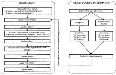
6.2.6 Model Im p le m e n ta tio n ... 99
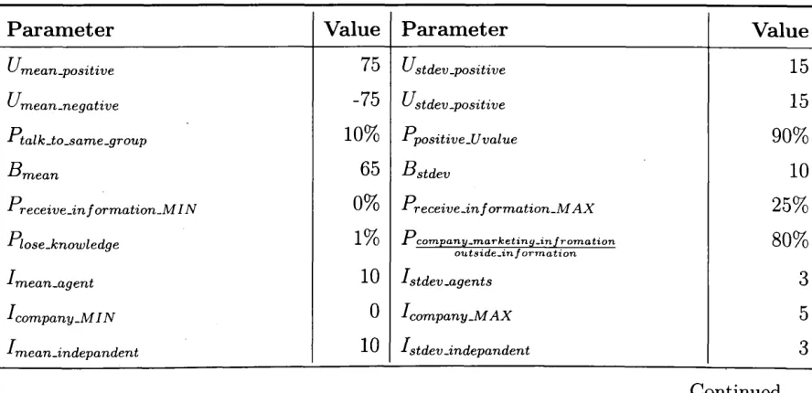
6.2.7 Default P a ra m e te rs ... 101
6.3 MODEL VERIFICATION & V A L ID A T IO N ... 104
6.3.1 Model Verification ... 104
6.3.1.1 Manual S im u la tio n ... 104
6.3.1.2 Excel S im u la tio n ... 105
6.3.1.3 STRESS T e s t ... 105
6.3.2 Model V a lid a tio n ... 106
6.4 O UTPU T V ALUES... 107
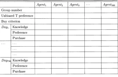
6.4.1 Main O utput File F o r m a t ... 107
6.4.2 Detailed O utput File F o rm a t... 107
6.5 S U M M A R Y ... 108
7 M O D E L B E H A V IO U R 110
7.1 MODEL BEHAVIOUR - BEHAVIOUR OF “REAL SYSTEM” . . . I l l
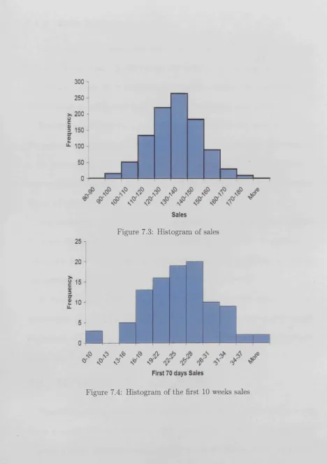
7.1.1 Sales D istrib u tio n ... I l l
7.1.2 Peer P r e s s u r e ... 114
7.2 SENSITIVITY ANALYSIS... 114
7.2.1 Experiment Parameters ... 116
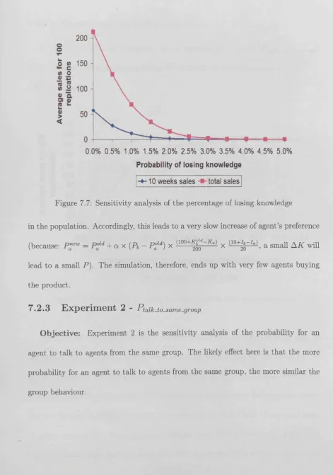
7.2.2 Experiment 1 - PloseJtnowledge... 117
7.2.2.1 Parameters Used in The E x p e r im e n t... 117
7.2.2.2 R e s u l t ... 117
7.2.3 Experiment 2 - Pialk.to.same.group... 118
7.2.3.1 Parameters Used in The E x p e r im e n t... 119
7.2.3.2 R e s u l t ... 119
7.2.3.3 Expansion - Peer Pressure T e s t ... 120
7.2.4 Experiment 3 “ P company-marke t mg-in fromation 121 outside-in formation 7.2.4.1 Parameters Used in The E x p e r im e n t... 121
7.2.4.2 R e s u l t... 121
7.2.5 Experiment 4 - B m ean... 122
7.2.5.1 Parameters Used in The E x p e r im e n t... 123
7.2.5.2 R e s u l t... 123
7.2.6 Experiment 5 - Umean.positjv e ... 124
7.2.6.1 Parameters Used in The E x p e rim e n t... 124
7.2.6.2 R e s u l t ... 124
7.2.7 Experiment 6 - K out and P out ... 125
7.2.7.1 Parameters Used in The E x p e rim e n t... 125
7.2.7.2 R e s u l t... 125
7.2.8 Experiment 7 - Group S iz e ... 126
7.2.8.1 Parameters Used in The E x p e r im e n t... 126
7.2.8.2 R e s u l t ... 126
7.3 S U M M A R Y ... 129
8 M O D E L C A L IB R A T IO N 131 8.1 SCENARIO IN V ESTIG A TED ... 132
8.2 CALIBRATION P R O C E S S ... 132
8.2.1 Parameters Used for C alib ratio n ... 132
8.2.2 Fitness C r i t e r i o n ... 133
8.2.3 Search Process ... 134
8.2.4 Search M e t h o d ... 136
8.2.5 Grid of Points ... 136
8.2.6 Initial Points for Initial Simplex S e a r c h ... 137
8.2.7 Nelder-Mead Downhill Simplex (Nelder and Mead, 1965) . . . 138
8.2.8 Nelder-Mead Searches ... 138
8.3 ‘EX PERIM EN T’ 1 (INITIAL PERIOD: 70 D A Y S ) ... 139
8.3.1 Grid of P o in ts ... 140
8.4.1 Grid of P o in ts ... 147
8.4.2 Initial Search P o i n t s ... 147
8.4.3' R e su lts... 149
8.5 EXPERIM ENT 3 (INITIAL PERIOD: 140 D A Y S ) ... 150
8.5.1 Grid of P o in ts ... 152
8.5.2 Initial Search P o i n t s ... 152
8.5.3 R e su lts ... 154
8.6 EXPERIM ENT 4 (INITIAL PERIOD: 175 D A Y S ) ... 156
8.6.1 Grid of P o in ts ... 156
8.6.2 Initial Search P o i n t s ... 157
8.6.3 R e su lts... 157
8.7 D IS C U S S IO N S ... 161
8.8 S U M M A R Y ... 162
9 C O N C L U S IO N S A N D F U T U R E R E S E A R C H 163 9.1 SUMMARY OF THE T H E S IS ... 163
9.1.1 Main A r g u m e n ts ... 163
9.1.1.1 Prediction, Model Calibration and the Inverse Problem 165 9.1.1.2 Approach Used in This R e s e a r c h ... . 166
9.2 RESEARCH OBJECTIVES AND CONTRIBUTION TO THE FIELD 166 9.2.1 Main O bjectives... 166
9.2.2 Secondary O b jectiv es... 167
9.3 FUTURE R E S E A R C H ... 168
9.4 FINAL C O N C L U S IO N S ... 169
A p p en d ices 171 A A B rief In trod u ction to A B S Packages 171 A .l List of agent-based simulation packages: Open S o u rc e ... 171
A.2 List of agent-based simulation packages: F re e w a re ... 174
A.3 List of agent-based simulation packages: Proprietary ... 175
B Search S im p lex 176 B .l Initial Period = 70 days ... 176
B.2 Initial Period = 105 d a y s ... 178
B.3 Initial Period = 140 d a y s ... 181
B.4 Initial Period = 175 d a y s ... 183
List o f Tables
2.1 Summary of general ABS model area derived from Reynolds (1999a) . 27
2.2 The existing ABS application a r e a s ... 28
2.3 Summary of ABS t o o l s ... 36
4.1 Key C o m p o n e n ts ... 75
4.2 Key C o m p o n e n ts ... 77
6.1 List of default p a r a m e t e r s ... 101
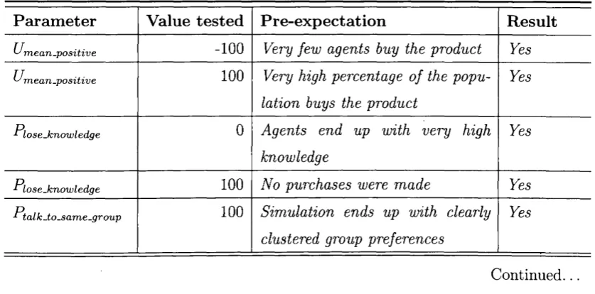
6.2 List of extreme param eters and tests’ r e s u l t s ... 105
6.3 Example of main model output f i l e ... 107
6.4 Example of model detailed output f ile ... 108
7.1 List of default p a r a m e t e r s ... 116
8.1 Grid param eter v a l u e s ... 137
8.2 Summary of the param eter searching r a n g e ... 139
8.3 Summary of the initial param eters for searching (70 days as initial period), note th at there were 6 points with 0 sales, so I arbitrarily picked one for L... 144
8.4 Search for Max Sales results with 70 days as initial p e r i o d ... 145
8.5 Search for Min Sales results with 70 days as initial p e r io d ... 145
8.6 The distance between the initial search points and search results . . . 145
8.7 Prediction range with 70 days as initial p e r i o d ... 146
8.8 Summary of the initial parameters for searching (105 days as initial p e r io d )... 149
8.9 Search for Max Sales results with 105 days as initial period ... 151
8.10 Search for Min Sales results with 105 days as initial p e r i o d ... 151
8.13 Summary of the initial parameters for searching (140 days as initial
p e rio d )... 154
8.14 Search for Max Sales results with 140 days as initial p e r io d ... 155
8.15 Search for Min Sales results with 140 days as initial p e r i o d ... 155
8.16 The distance between the initial search points and search results . . . 155
8.17 Prediction range with 140 days as initial p e r i o d ... 156
8.18 Summary of the initial parameters for searching (175 days as initial
p e r io d )... 159
8.19 Search for Max Sales results with 175 days as initial p e r io d ... 160
8.20 Search for Min Sales results with 175 days as initial p e r i o d ... 160
8.21 The distance between the initial search points and search results . . . 160
8.22 Prediction range with 175 days as initial period ... 160
List o f Figures
1.1 Thesis S tru c tu re... 6
2.1 Contents of Chapter 2 ... 10
2.2 Rogers adoption innovation curve (Rogers, 1962) 16 2.3 The Environment-Rules-Agents framework to build agent-based com putational models (Gilbert and Terna, 2 0 0 0 ) ... 33
3.1 Contents of Chapter 3 ... 38
3.2 Issue with black box validation ... 44
3.3 ABS model validation (Derived from Moss, 2000) ... 45
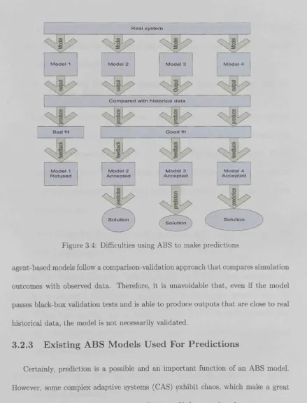
3.4 Difficulties using ABS to make p r e d ic tio n s ... 49
4.1 Contents of Chapter 4 ... 63
4.2 Rogers adoption innovation curve(Rogers, 1 9 6 2 ) ... 68
4.3 Bipartite network m o d e l ... 79
4.4 Random social n e tw o rk ... 80
4.5 Small social n e t w o r k ... 80
5.1 Flow chart of the proposed m e th o d o lo g y ... 83
6.1 Interactions in the m o d e l... 92
6.2 How agents change their knowledge and p re fe re n c e s... 94
6.3 Objects: agent and source in f o r m a tio n ... 100
6.4 Group size d is trib u tio n ... 103
7.1 The product life cycle as measured by average number of buyers over 1000 simulation r u n s ... 112
7.2 The cumulative sales(average of 1000 r u n s ) ... 112
7.5 Grouped agent’s preference... 115
7.6 Purchase rate for each g r o u p ... 115
7.7 Sensitivity analysis of the percentage of losing k n o w led g e ... 118
7.8 Probability for agent to talk to agents from the same g ro u p ... 119
7.9 The group uptake percentage ... 120
7.10 Probability for agent to receive outside marketing information . . . . 122
7.11 The mean of agent’s buying c r i t e r i o n ... 123
7.12 The normal distribution mean of agent’s unbiased true preference . . 124
7.13 Scatter of sales, company knowledge and company preference... 127
7.14 Scatter of sales, company knowledge and company preference... 127
7.15 Sensitivity analysis on the social group s iz e ... 128
7.16 Sensitivity analysis on the social group s iz e ... 128
8.1 Contents of Chapter 8 ... 131
8.2 Extrem a of a function in an interval (based on Press et al., 1992) . . 135
8.3 Model calibration process ... 136
8.4 Contour map of the total s a le s ... 142
8.5 Contour map of the fitness (initial period: 70 d a y s ) ... 142
8.6 Histogram of the sales values for the 40 points with fitness 0 ... 143
8.7 Histogram of the sales values for the 35 points with fitness 0 ... 148
8.8 Contour map of the fitness (initial period: 105 days) ... 148
8.9 Histogram of the sales values for the 27 points with fitness 0 ... 153
8.10 Contour map of the fitness (initial period: 140 days) ... 153
8.11 Histogram of the sales values for the 23 points with fitness 0 ... 158
8.12 Contour map of the fitness (initial period: 175 days) ... 158
8.13 Prediction Range Vs Information available... 161
A b stract
Agent-based simulation is increasingly used to study systems in many areas of
business and science nowadays. Agent-based simulation refers to simulations of sys
tems th a t contain agent entities whose behaviour depends dynamically on the state of
the system. This enables the agents to adapt their behaviour to changing conditions.
For some applications, using agent-based simulation for prediction (rather than just
for a better understanding) could be very powerful. For example, a company might
wish to use a model of the population of their customers with word-of-mouth inter
actions to predict the sales of their product or the effect of an advertising campaign.
However, the problem is th a t agent-based models typically have a very large num
ber of param eters and many of these cannot be measured directly or estimated with
sufficient precision.
The result is th at a wide range of sets of param eter values may give an acceptable
fit and are therefore feasible values. However, they may give quite different predic
tions. Therefore, simply choosing a single set of param eter values th at produces a good
fit may mean th a t the model results are incorrect and very misleading. The inverse
problem has been studied in other areas of science including groundwater modelling
(Brooks et al., 1994), but it appears th a t this issue has not yet been investigated for
agent-based simulation.
In order to investigate the extent of this problem, in the research an agent-based
consumer diffusion model was developed and treated as the real system. Selected
output d ata from this model was used as measured values from the real world. In a
pseudo-modelling exercise, this d ata was then used to calibrate agent-based models
of the system, and a method similar to th a t of Brooks et al. (1994) was used to find
the extent of the variations in predictions. The method had to be adapted since the
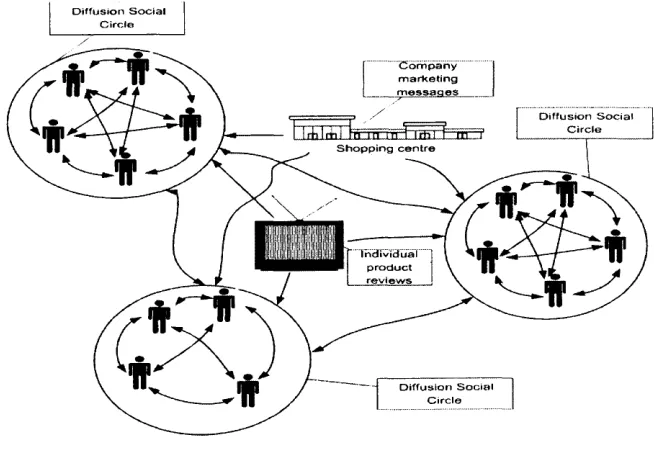
than a vast population of agents with many neutral contacts is represented. All
agents are allocated to a diffusion social circle with a certain level of influence within
the social network. These are constant attributes for th a t individual throughout the
simulation. All agents initially have no knowledge or preference about the selected
product. During the simulation, agents receive marketing communication messages
(i.e. from company’s advertisements, supermarkets, online search results etc.) and
contact each other to exchange their knowledge and preferences about the product.
There has been very little agent based modelling of this situation and the mechanisms
developed represent a potential theoretical structure for this application. Sensitivity
analysis was carried out and the model appears to produce realistic behaviour.
The adapted method was applied to four experiments of different amounts of
observed d ata (initial periods of 70, 105, 140 and 175 days) to find the range of
predictions of total sales in each case. The total sales for the real system model were
124 and the range of predictions for the four experiments were [58, 376], [79, 319], [91,
277], [109, 187]. As expected, the prediction range narrows as more d ata is available.
However, the range of predictions is very wide for all four experiments and therefore
the model would have limited usefulness for predicting sales in this type of situation.
In particular, choosing a single set of param eter values is not appropriate and could
A cknow ledgem ents
Great thanks to Dr. R oger B rooks, my super supervisor, who guided me through
out the simulation world, for his patience and constant support during this research.
I cherish the love th at my parents have generously, continuously given to me at all times. W ithout them, this work would never have come into existence (literally).
Finally, I wish to thank my dear friends: Dr. Z hen L iu, Dr. H on gyan L i, Dr.
W ang W ang, Q ian xin M u, my lovely “Russian comrade” : Dr. A le x ey A r to m o n o v,
“Portuguese lady” : Dr. A d e la id e C arvalh o and “Jamaican brother” : Dr. N ich olas
P e a rso n for their wonderful friendship.
Some of the thesis published as papers presented in conferences.
IN T R O D U C T IO N
1.1
IN TRO DUCTIO N
In recent years, agent-based (or individual-based) simulation has received a lot
of attention. Agent-based simulation refers to simulations of systems th a t contain
agent entities whose behaviour depends dynamically on the state of the system. This
enables the agents to adapt their behaviour to changing conditions. In modelling such
adaptive behaviour, agent-based simulation as a tool is commonly used in complexity
science (Waldrop, 1993).
There is no standard definition of an agent. Some definitions list a set of prop
erties, but a better approach is perhaps simply to say th at an agent is an entity for
which some cognitive process is modelled (Edmonds and Mohring, 2005). Usually,
agents receive information from the environment (including other agents) and have
internal rules th a t represent the cognitive decision process and determine how they
respond. The rules can be a simple function of the inputs received or can be very
complex incorporating various internal state parameters, which can include a model
representing the agent’s worldview of some part of the environment (such as predic
2
processes is the PECS model, which has a hierarchical structure with states for physic
(physical body), emotion, cognition and social status as well as sub-components for
each of these (Schmidt and Schneider, 2004).
In some cases, the rules governing the agents’ behaviour are fixed throughout the
simulation, while in other cases, the rules can change to represent learning. The
number of agents modelled can also vary from an individual agent through to a large
population. Populations are usually heterogeneous with individual agents having dif
ferent parameters or even quite different rules (e.g. different trading strategies in a
stock-market simulation). Interactions between the agents are often a key part of
the behaviour of the system. A very wide variety of applications have been stud
ied using agent-based simulation, including stock markets, auctions, the spread of
disease, ecosystems, military battles, crowd dynamics, sports games, transport, so
cial behaviour, social networks, the development of technology, and consumer market
behaviour (such as fads). For instance, the agents might represent stock brokers
in stock markets, bidders in an auction, disease cells, autonomous characters in com
puter games, vehicles in traffic, chunks of code in software, people in crowds, economic
regimes, or plants and animals in ecosystems.
For some applications, using agent-based simulation for prediction (rather than
just better understanding) could be very powerful. For example, a company might
wish to use a model of the population of their customers with word-of-mouth inter
actions to predict the sales of their product or the effect of an advertising campaign.
However, the problem is th at agent-based models typically have a very large num
sufficient precision. The only other information available may be historical output
data from the real system. Such d ata can be used to calibrate the model by finding
param eter values th a t produce a good fit with the data. This is known as an inverse
problem since it consists of using the outputs to determine the inputs. The problem
is th at there will usually be many solutions. There are two main reasons for this.
The first is th at there are often many param eters and few historical data values. The
second is th a t any model th a t produces a good fit could be considered acceptable. A
perfect fit is not expected because any simulation is a simplification of the real system
and also there may be measurement errors in the historical data.
The result is th at a wide range of sets of param eter values may give an acceptable
fit and are therefore feasible values. However, they may give quite different predic
tions. Therefore, simply choosing a single set of param eter values th at produces a good
fit may mean th a t the model results are incorrect and very misleading. The inverse
problem has been studied in other areas of science including groundwater modelling
(Brooks et al., 1994), but it appears th a t this issue has not yet been investigated for
agent-based simulation. An im portant difference between agent-based simulation and
groundwater modelling is th at agent-based simulation models are stochastic where
groundwater models are deterministic.
The complex non-linear nature of most simulation models means th a t there is no
simple equation for the feasible values of the parameters. Therefore, methods used
for tackling the inverse problem have involved running the simulation and deriving
alternative predictions in some way from those runs.
4
• Calibration problem: The problem of obtaining the values of parameters that
cannot be measured directly. This requires a calibration process using output
data, which is an inverse problem.
• Inverse problem: Generally refers to problems where the answer is known but
the question is unknown, and so knowledge of the answer is used to find the
question. In this case, the process of using output d ata to determine model
inputs, by finding param eter values th a t give model output th at is (dose to the
observed output values.
• Prediction problem: The problem of using a model to make predictions when
there is uncertainty as to the param eter values. The different param eter values
th a t give a good fit can produce a wide range of predictions and so the process
of making predictions needs to take this into account.
This research sets out an approach, which is explained in the following chapters,
to investigate these problems further for agent-based simulation by developing a con
sumer word-of-mouth model and searching for the range of predictions th at arise from
alternative acceptable calibrated param eter values.
1.2
RESEARCH OBJECTIVES
1 .2 .1 M a in O b je c tiv e
The main objective of the research is to investigate the effect of obtaining the
param eter values of an agent-based model by calibration when using the model for
• developing and implementing a method based on previous research for obtaining
an acceptable range of predictions from the alternative acceptable calibrations.
• comparing the range of predictions for different scenarios of the data available
for calibration.
1 .2 .2 S e c o n d a r y O b je c tiv e s
The system studied in the research is consumer word-of-mouth (WOM) inter
actions. Few agent-based models have been built of this situation and there is no
consensus as to the best way to model the agents or the interactions. Therefore, a
secondary objective is to contribute towards modelling in this area by:
• developing a new agent-based WOM consumer model
• investigating the relationships between the param eters and the model output
• assessing whether the model produces realistic output.
1.3
BRIEF OVERVIEW OF APPR O A C H
The approach used was to develop an agent-based model and to treat this model
as the real system. O utput data from this model could then be taken as measured
values from the real world and, in a pseudo-modelling exercise, used to calibrate an
agent-based model of the system. The advantage of such a pseudo-modelling exercise
is th a t the “real system” is completely known. Consequently, the model’s predictions
can be compared with the “true” future values, and the precise differences between
6
1.4
THESIS STR UCTURE
Figure 1.1 shows the structure of the thesis and how the chapters contribute to the
problem being investigated. Chapters 2, 3 and 4 set the work in context by reviewing
previous literature, while Chapter 5 set out the research methodology. Chapter 6 ex
plains how the model used in the research works. Chapter 7 describes experiments, to
understand the behaviour of the model, including sensitivity analysis. Chapter 8 de
scribes the implementation of the calibration method. Finally, Chapter 9 summarises
the contents of the thesis and describes possible future research.
c o 03 N ‘ c 03 03 CO CO 0 S I h
-Introduction Chapter 1
Introduction Literature Review
Research
Background Chapter 2 Agent- based
Simulation
Chapter 3 Calibration Of
Agent-based Simulation Models
Chapter 4 Agent-based Diffusion Models
Research methodology
Chapter 5 Methodology
Model
Framework Chapter 6 Customer Diffusion
Model
Chapter 7 Experiments
Chapter 8 Model Calibration
Conclusions Chapter 9
Conclusions and Future Research
[image:21.461.4.453.145.738.2]The following sections give an overview of each chapter.
C h a p te r 2
Chapter 2 provides a context for the rest of the thesis and discusses a range of
ideas relevant to the validation of agent-based models. It defines complexity, complex
adaptive systems and agent-based simulation (ABS). It identifies the main theoretical
and methodological perspectives of ABS, and reviews recent work and key themes of
discussion and debate in this field. In addition, this chapter reviews currently used
agent-based simulation software packages and provides a brief introduction to each
one.
C h a p te r 3
Chapter 3 reviews relevant literature on the calibration issue in agent-based sim
ulation models, which is the main research topic of the thesis. The chapter defines
ABS model validation and verification, prediction in agent-based simulation, the in
verse problem, the param eter identification problem, and best-fitting parameters. It
introduces some existing calibration methods, namely the Bayesian MCMC based
method and the range prediction method. It also discusses current model-calibrating
methods. To conclude the chapter, two applications using an ABS model for predic
tion are introduced.
C h a p te r 4
C hapter 4 reviews the existing agent-based models th a t have been used to inves
customer relationship management (iCRM) model from BT and the J-pop agent-based
prediction model. It also briefly introduces the classic 1969 Bass diffusion model,
which has now become the fundamental theoretic frame of most diffusion models.
The chapter concludes with a discussion of the advantages and disadvantages of each
of the above models.
C h a p te r 5
Chapter 5 illustrates the research methodology used in the research through a
step-by-step simulation modelling plan for the research. In the end of the chapter, it
gives a discussion of the advantages and disadvantages of the approach used in the
research.
C h a p te r 6
Chapter 6 describes the model (an agent-based consumer word-of-mouth model)
used to conduct the research. It introduces the model’s structure (including agents’
environments, agents’ attributes and how agents’ interactions will change one an
other’s attributes), the model’s param eters and the model’s procedure. It also details
the model’s validation and verification, and describes a manual simulation and an
Excel-based formulation used to verify the model.
C h a p te r 7
Chapter 7 describes some experiments conducted to understand the way the model
behaves. It starts with the model output study to give a general idea of how the
to investigate the impacts of various parameters, including the probability of losing
knowledge at the end of each simulation day, the probability of an agent talking to
agents from the same group, the probability of an agent receiving outside marketing
information, the mean in the normal distribution of an agent’s buying criterion and
the mean in the normal distribution of an agent’s unbiased true preference. An
experiment on the knowledge and preferences of the outside marketing sources were
also undertaken. Additionally, the number of agents in each group was varied.
C h a p te r 8
Chapter 8 demonstrates the step-by-step implementation of the calibration method
used in the research on the agent-based WOM model. By adopting a similar method
to th a t of Brooks et al. (1994) for searching for param eter sets th a t fit the model, the
model used in the research shows a big prediction range in a variety of scenarios. It
concludes th a t a calibrated model can still produce a big range of prediction and a
careful calibration is needed to qualify the use of agent-based simulation models for
prediction .
C h a p te r 9
Chapter 9 summarises the contents of the thesis and discusses the results of ex
periments, how these met the objectives of the research as set out in Chapter 1, the
C h a p ter 2
A G E N T -B A S E D SIM U LA TIO N
Chapter Overview
Complexity World
Complexity CAS Why ABS
ABS MAS What is an agent
ABS features comparing with traditional simualtion
ABS applications
ABS Tools Graphically representation of ABS
List of ABS tools
ERA UML
Figure 2.1: Contents of Chapter 2
This chapter provides a context for the rest of the thesis and discusses a range
of ideas relevant to the validation of agent-based models. It defines complexity, the
complex adaptive system and agent-based simulation (ABS). It identifies the main
theoretical and methodological perspectives of ABS and reviews recent work and key
themes of discussion and debate in this field.
S e c tio n 2.1 gives an introduction to the world of complexity and complex adap tive systems, which highlights the point th a t agent-based simulations are suitable for
studying complex adaptive systems.
S e c tio n 2 .2 describes the key features th at an agent should have and explains the procedure of agent-based simulation as a modelling technique. It also compares agent-
based simulation with traditional simulation. S e c tio n 2 .3 introduces the graphical
representation methods for the ABS model (e.g. ERA and UML). It also summaries
the main ABS modelling tool kits.
2.1
Introduction to the World of Com plexity
2 .1 .1
W h a t is C o m p le x ity ?
2.1.1.1 C o m p lex ity
Nowadays, complexity is a fashionable and popular topic. Generally speaking,
complexity theory attem pts to answer the questions th a t in the past have been con
sidered as impossible tasks because of the lack of advanced techniques, computational
power and associated complexity. However, with the development of experimental
technology and com putational power, scientists have been able to study certain as
pects of the complex world, and complexity theory has been applied to a variety of
existing domains, such as stock markets, auctions, the spread of disease, ecosystems,
military battles, crowd dynamics, sports games, transport, social behaviour, social
networks, the development of technology, and consumer market behaviour (such as
12
2.1.1.2 F ingerp rin ts o f T h e C om plex
The following are a few of the most im portant “Fingerprints of the complex”
recognized by Casti (1997):
• Instability: Complex systems tend to shift between many possible modes of
behaviour, and the whole system can be affected dramatically by small changes
(such as the “tipping point”).
• A dap tab ility: Agents in the complex system are sometimes able to change
their decision rules on the basis of partial information about the entire system.
• Irred u cib ility/E m ergen ce: The complex system should be studied as a uni
fied system. In other words, the behaviour of the system is determined by
interactions among agents, so th a t it cannot be studied by looking at agents
in isolation. Therefore, complex systems produce surprising outputs/behaviour.
In other words, system behaviour patterns and properties cannot be predicted
easily via individuals’ rules of behaviour.
• M em ory: Complex adaptive systems have memory, which is distributed through
out the whole system instead of being located at a specific place. The whole
system behaviour is related to the system history.
• C onn ectivity: The complex system’s elements are connected and interactive.
W hat makes a system a system and not simply a collection of elements are the
connections and interactions of the individual components of the system, as well
Among the above fingerprints of the complex, Casti (1997) argues th a t the most
distinguishing single feature of the complex system is “emergent behaviour” . The
appearance of the “emergent behaviour” is related to the whole system history be
haviour and mainly due to the interaction between system parts. However, the system
output is not usually predictable by analyzing separate system parts.
From the late 20th century, researchers began to explain this “emergent behaviour”
as the result of non-linear world around us. In the nonlinear systems, it was found
th a t capturing the exact rules/equations of their behaviour is sometimes of little
help in predicting system outcomes. Real-world systems, especially those involv
ing people, are generally too nonlinear to predict (Lucas, 1999). Researchers have
found th a t the traditional theory was limited in terms of interpreting such Complex
Adaptive Systems (CAS). They define the essence of CAS th a t they self-organise to
improve/optimize the objective function and the system behaviour depends on the
interactions of system parts (Lucas, 1999; Casti, 1997). Furthermore, Casti (1997)
summarizes a number of characteristics he describes as the “Key Components” of
CAS, namely:
• M ed iu m -sized num ber o f agents: The number of agents must be neither
so small th a t all their interactions could be worked out very easily, nor so large
th a t statistical aggregation methods could answer most kinds of questions about
the system.
14
they are capable of responding to external changes with the help of in-built be
haviour rules and forming their self-maintaining systems with internal feedback
paths.
• L ocal inform ation: No agent has perfect information about the whole system.
The agent only has “local” or “partial” information. In other words, there is no
agent in the system who knows what every other agent is doing. Therefore, in
the system, agents are making their decisions based on limited information.
We can take ecosystems as a typical example to examine the above key points
of CAS. In an ecosystem, the system patterns emerge from “localized interactions
and selection processes acting at lower levels. An essential aspect of such systems
is nonlinearity, leading to historical dependency and multiple possible outcomes of
dynamics” (Levin, 1998). In other words, in ecosystems, knowing a single species
behaviour rule does not help with predicting the whole system emergent pattern. Such
patterns arise from the interactions between species and are related to the system’s
previous statu s/p attern .
2 .1 .2
T ip p in g P o in ts
Gladwell (2002) brought the term “tipping point” into CAS to describe the afore
mentioned “emergent behaviour” in a social context. The tipping point is a sociolog
ical term th a t refers to “the moment when something unique becomes common.” For
instance, a tipping point could refer to the moment of an epidemic outbreak (e.g. the
dram atic moment in an epidemic when everything changes all at once), boiling point,
the following five key concepts of tipping point:
T h e Law o f th e Few Among the whole population, there are some people with
much higher influence than others. Also, these people are willing to spread the
information of social phenomena through a population. W ithout their aid, the
“tipping point” is unlikely to occur.
T h e S tick in ess Factor Messages about the new ideas or products must be found
attractive or interesting by others (i.e. easy to remember, attractive for people
to move to action.).
T h e Pow er o f C o n tex t Gladwell claimed th a t human beings are more sensitive to
their environment than they seem to be. The context changes can sometime tip
an epidemic unexpectedly.
T h e M agic N u m b er 150 Some researchers suggest 150 is the maximum number of
people which an individual can have social relationships with (Dunbar’s num
ber1).
T h e N ew P ro d u ct C ycle In an adoption innovation model ( Figure 4-2), Rogers
(1962) presented a bell curve of adaptation to a new phenomenon. When a new
product was put into the market, the adopters were categorized into five groups
based on their attitudes to the new product, namely: innovators, early adopters,
early majority, late majority, and laggards. According to Roger’s research, the
16
m ajority adopters are “early m ajority and late m ajority” which accounted for
64 % of the population.
C/2 Uh Oh O < o 4> OD ■2c <L> O I— 4> Ph
E a rly M a jo r ity
14% E a rly
A d o p te r s 1 3.5%
L a te M a jo r ity
3 4% I n n o v a to r s
2.5%
A d o p t e r s ’ C a t e g o r i e s b a s e d o n I n n o v a t i v e n e s s
Figure 2.2: Rogers adoption innovation curve (Rogers, 1962)
2 .1 .3
W h y is A g e n t-b a s e d S im u la tio n S u ita b le t o S tu d y C A S ?
The aim of simulation in general, is to gain insight into the systems th at people
do not completely understand. Agent-based simulations enable and aid the under
standing of complex systems. Agent-based simulations are suitable for the study of
CAS because the model is based on simple rules or algorithms by which the agents
within a population behave, instead of the almost impossible task of building a mass
detailed model where all interactions between agents and their effects are mapped
out. Furthermore, three main reasons for adopting agent-based simulation to study
CAS are:
• Medium number of agents: As mentioned above, with medium-sized numbers
• Complex interactions: Because of the complex and sometimes nonlinear, and
discontinuous interactions between the heterogeneous agents, the behaviour of
the system as whole is difficult to predict based on individual’s behaviour. Tra
ditional analytic techniques cannot cope with the complex interactions of CAS
(Bonabeau, 2002a). T hat is also one reason why analytical tools have not been
widely used in social science before.
• Intelligent and adaptive agents: When agents exhibit complex behaviour includ
ing learning and adaptation, they can be more easily represented as computer
programs than with other traditional methods.
These features will be explained more with applications in S e c tio n
2.2.4-2.2
Agent-based Simulation as a Young Field
Agent-based simulation is still a young and rapidly growing field. This section
presents the findings of an extensive review of ABS literature. It also introduces some
ABS applications to provide a general idea of how and in which fields ABS could be
applied.
2 .2 .1
M u lti-A g e n t S y s te m s (M A S )
The agent concept was originally developed from MAS (multi-agent system). A
multi-agent system is usually considered as a collection of “solving systems capable of
autonomous reactive, pro-active, social behaviour” (Lomuscio, 1999). These solving
systems work together to find the solution (Durfee et al., 1989). In this context,
18
Recently, MAS has been given a more general meaning. It refers to all systems which
involve agents (as defined in the following section) (Jennings and Wooldridge, 1998).
And the study of MAS focuses on systems in which many intelligent agents interact
with each other.
2 .2 .2
W h a t is an A g e n t?
Recently, agent-based simulation has become a commonly used term in the simu
lation literature. However, agreement on the precise definition of agent-based simu
lation has been difficult to achieve. Edmonds and Mohring (2005) gave the definition
of an agent as an entity for which some cognitive process is modelled. Tunce (2001)
defines agent-based simulation as the “use of agents for the generation of model be
haviour in a simulation study” . Reynolds (web page) says th a t “agent-based models
are simulations based on the global consequences of local interactions of members of
a population” . Actually, none of these definitions contributes much towards a better
understanding of agent-based simulation. However, Dickie (2002) tells us more about
agent-based simulations; he states th a t “in agent-based simulation models, an entity’s
behaviour is generally modelled as a set of goals or actions. Agents control their own
destiny, or in other words change their state based on their knowledge of the envi
ronment in which they are placed” . From these different definitions of agent-based
simulation, it is clear th a t the key to agent-based simulation is the agent notion. Such
individuals (agents) might represent vehicles in traffic, plants and animals in ecosys
tems, chunks of code in software, autonomous characters in computer games, people
In agent-based modelling, several authors have tried to identify the key aspects of
an agent. Holland (1995) defines agents as “rule-based input-output elements whose
rules can adapt to an environment” . Dickie (2002) says th a t the character of an agent
is th a t once an agent’s knowledge has been built, the “behavioural mechanism acts
on its degrees of freedom” . An agent’s degrees of freedom are the state variables the
agent is able to affect. An agent’s behaviour is a function th at takes knowledge as an
input, and outputs changes to the agent’s degrees of freedom. A more comprehensive
definition of an agent is given by Weiss (1999). He states th a t an agent is “a compu
tational entity th a t can be viewed as perceiving and acting upon its environment and
th a t it is autonomous in th a t its behaviour at least partially depends on its own ex
perience” . Rocha (1999) takes the view th a t the distinctive characteristic of agents is
their autonomy, which means th a t an agent has the ability to act and make decisions
without being controlled. Moreover, Schmidt (2000) and Holland (1995) review the
features of agents, which will be discussed in the following parts:
Schmidt (2000) reviews the features of agents as the following aspects:
1. Autonomous behaviour: “Every agent is characterized by autonomous behaviour” ,
e.g. an intelligent agent behaves autonomously without external control.
2. Individual world-view: Every agent perceives its surrounding external world
according to its own model. This so-called conceptual model describes the
intelligent agents’ view of the outside world, and it is generally incomplete and
frequently even incorrect.
20
exchange between intelligent agents and their environment, which may consist
of other intelligent systems and even other intelligent agents. Thus, intelligent
agents exchange information with the external environment and with other in
telligent agents in order to build up their own world view. In addition, the
possibility of communication with other intelligent agents is the “precondition
of common action in pursuit of a goal” .
4. Intelligent behaviour: Agents are able to learn from the environment, as they
have the capacity of “logical deduction” . Therefore, intelligent agents can be
used in unknown environments.
5. Spatial mobility: Intelligent agents are sometimes but not always required to
display spatial mobility. (Spatial mobility is not included in the model in this
research.)
On the other hand, Holland (1995) defines seven “basics” or characteristics of
agents:
1. Aggregation.
• Categorization (agent-level): In order to cope with their environments,
agents group things with common characteristics and ignore differing char
acteristics.
• Large-scale behaviour (multi-agent level): The collective behavioural p at
terns emerge from the aggregation of the individual agents’ behaviour.
3. Nonlinearity. In a multi-agent system, the integration or aggregation of agents
is often non-linear. Thus, the resulting behaviour cannot be linearly predicted
by decomposing the behaviour of individual agents.
4. Flows. The ABS relies on the connections (e.g. the flow and transfer of infor
mation, interactions etc.) between agents.
5. Diversity. Because MAS are designed to play different roles, multi-agent systems
are typically heterogeneous. However, the agents’ behaviours may be identified.
6. Internal Models. Every agent has its own internal model. The internal model
organizes the individual agent’s behaviour rule and can also enable agents to
anticipate the expected inputs from their environment.
7. Building Blocks. Agents are built with simple components which make the
coded construction easier. Therefore, model users can recombine the agents to
produce a new agent with different behaviour and models.
Holland’s basics give more emphasis to the emergence of large-scale behaviour or
a multi-agents level (points 1,3,4,5), whereas Schmidt only mentions group behaviour
in one point (point 3). Holland’s basics are more comprehensive than Schmidt’s and
his paper also considers each part in great detail and has been widely cited. However,
Schmidt’s characteristics and Holland’s basics share some common features; on one
hand, they both agree th at agents have their own internal models, i.e. they both
have individual views of the world and rules of behaviour; on the other hand, they
22
as a simulation based on the global consequences of local interactions of autonomous
intelligent members of a population (Reynolds, 1999a). In addition, an agent is an
individual with a set of characteristics or attributes, a set of rules governing agent
behaviours or decision-making capability, protocols for communicating responses to
its environment and th at interacts with other agents in the system.
2 .2 .3
A B S V s T r a d itio n a lly S im u la tio n
Is agent-based simulation some new, fancy way of doing analysis? Is agent-based
simulation just old wine in a new bottle? Although agent-based simulation is some
times presented as if it were a new type of modelling, many “traditional” simulations
feature some adaptive agent behaviour. For example, a simple queueing simulation
may include a rule th at customers (the agents) will not, with some probability, join
the queue if its length exceeds a certain value, or th a t customers leave the queue if
they have to wait too long.
In order to compare traditional simulation and ABS, the main typical character
istics (with some exceptions) are considered to be:
Typical characteristics of traditional simulation (examples: production line, call
center, hospital, transport system):
1. The systems is one of queues and processes and so the main elements are the
processors, the queues and the processed elements.
2. The range of behaviour of the processors is processing time and the next desti
3. The item being processed (e.g. parts, customers, vehicles) is often passive al
though it may have heterogeneous characteristics.
4. The connections between the processors and queues (the flows through the sys
tem) are designed (top down) in the real system and so are focused in the
simulation.
5. The stochasticity occurs in the arrivals of the element being processed, the
processing times and sometimes the characteristics of the processed element,
and the rules of the processed element.
6. Typical outputs of interest are throughout, queueing time and resource usage.
Typical characteristics of agent-based simulation (examples: stock market, auc
tion, consumer market, military battle, crowds and epidemics):
1. The system is one of interacting agents and so the main elements are the agents
and the environment.
2. There is a variety of behaviour of agents depending on current circumstances.
3. The agents have heterogeneous characteristics and rules of behaviour.
4. The agents’ characteristics may change during the simulation (e.g. a change in
strategy, an increase in knowledge, become ill or die).
5. The interactions between the agents are not designed but are unpredictable and
24
6. The stochasticity occurs in the characteristics of the agents and their rules, the
interactions between the agents and the interactions between the agents and the
environment.
7. The item th a t passes between the agents (information, opinions, disease) is often
intangible and its impact on the receiver depends upon the characteristic of the
receiver.
8. Typical outputs of interests are aggregated agent behaviour (e.g. number of
purchases, number of agents in different states) or the state of the environment
(e.g. market price).
We can view both traditional and agent-based simulations as consisting of entities
th a t remain in the system throughout the simulation and interactions between the
entities through elements th a t between them. Viewed in this way, the corresponding
entities remaining in the simulation are the processing entities and queues in tra
ditional simulation (e.g. machines, servers), and the agents in ABS. Moreover, the
elements passing through the connections between the entities are of a different nature
as highlighted in the above list of characteristics. In traditional simulation, it is often
a physical element th at passes from one entity to the next w ithout altering the enti
ties (although sometimes information can be passed). The physical element usually
follows a route through the system. In ABS, the agents exchange elements th at alter
their characteristics and the elements are just involved in separate transactions rather
than following a route between several agents.
based consumer model (where consumers exchange information and opinions about a
product and ultimately purchase the product). Because in both cases, the elements
remaining in the system are human beings and the systems centre around conversa
tions. However, in the call centre, the conversations between the customer and the
operator are modelled as simply a processing task which does not alter the character
istics of the customers or operators. The im portant data is the distributions for the
call inter-arrival times and the processing times. In the consumer model, the precise
time at which the conversations between the agents take place and the length of time
of the conversations are not im portant. Instead it is the number of conversations and
the way they affect the characteristics of the agents th a t matters.
Complexity and unpredictability in simulation behaviour usually arises mainly
from the stochasticity. In traditional simulation, the most, significant aspect is typ
ically the time taken by the processed element as it passes through the system (i.e.
arrival time and processing time). There can also be stochasticity in the characteris
tics and rule of the processed element. In agent-based simulation, the most significant
aspect is typically the characteristics of the agent and the interaction between the
agents. Therefore, the site of the stochasticity is different being related mainly to the
processed element in traditional simulation (the characteristics and time) but being
related mainly to the entities remaining in the system (i.e. the agent) in ABS.
In terms of applications, the systems studied by traditional simulation are often
designed by an organisation to accomplish a particular task and they have a lot of
control over the system. By contrast, the systems studied by ABS are often envi
26
environment). In such a situation, if there is an organisation with an objective (e.g.
a company wants to maximise sales in the consumer market), then they have very
limited control or influence over the system.
Overall, there are some differences between traditional simulation and ABS in the
amount of control exerted on the real system, on the nature of the elements modelled
and the way they interact, on the site of the stochasticity in the model and in the
aspects of interest. It is arguable how fundamental these differences are although I
would not consider them great enough for ABS to be considered as a new paradigm.
One of the causes of the greater use of agent-based simulation is th at increasing
computing power now makes such simulations feasible. There is also an appreciation
th a t for some systems an agent-based approach may be necessary in order to capture
the dynamics of the system.
2 .2 .4
O v er v ie w o f A B S A p p lic a tio n A r ea s
Quite a lot of research has recently been undertaken to apply agent-based sim
ulations in various fields, including psychology and cognitive science, ecology and
environment, economics and industry. Accordingly, there are a huge number of ap
plications in the literature. For instance, the academic paper and book search-engine
“google s c h o la r” returned 5,780 results for the search phrase “agent-based simulation” (last access date 06/10/2007). Therefore, in this section, some examples will only be
described at a level of detail intended to give an impression of the scope of the ap
plication areas. More details and examples can be found by consulting the literature
detail in the following chapters.
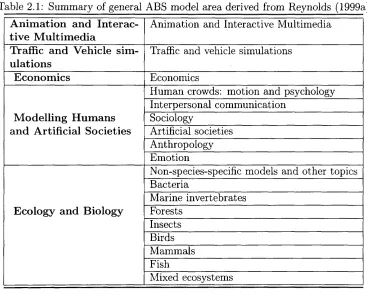
A comprehensive annotated list of ABS application areas is provided by Reynolds
(1999a), as summarized in Table 2.1. Consulting Reynolds’ (1999) list and other liter
ature, we can take the following four general topic areas to introduce a few examples
of the application of the ABS model (see Table 2 .2 and the following subsections).
Table 2.1: Summary of general ABS model area derived from Reynolds (1999a)
A n im a tio n and Interac tiv e M u ltim ed ia
Animation and Interactive Multimedia
Traffic and V ehicle sim u lation s
Traffic and vehicle simulations
E conom ics Economics
M od ellin g H um ans and A rtificial S o cieties
Human crowds: motion and psychology Interpersonal communication
Sociology
Artificial societies Anthropology Emotion
E cology and B io lo g y
Non-species-specific models and other topics Bacteria
Marine invertebrates Forests
Insects Birds Mammals Fish
Mixed ecosystems
2.2.4.1 M ovem ent P a ttern s
Boids (a contraction of bird and android) simulation (Reynolds, 1987) is one of
the earliest examples of applying an agent-based approach to a situation th at was
previously considered very difficult (O ’Sullivan and Haklay, 2000). Reynolds tries to
[image:42.465.45.412.197.489.2]28
Existing ABS application areas
Movements ABS models
Economics ABS models
Sociological ABS models
Military ABS models
Table 2.2: The existing ABS application areas
rules for general agents (boids) to produce behaviour th a t appears realistic compared
to the flocks, herds and schools of different animals in the real world. More agent-
based models th a t are aiding researchers investigating biological phenomena can be
found in Levy (1992), Resnick (1994) and Westervelt and Hopkins (1999).
Similar to the “Boids” model, a number of ABS models have been applied to the
study of human movement (Bonabeau, 2002a), such as:
P ed estria n and crowd behaviou r The “STREETS” model of people’s shopping
behaviour by Schelhornet al. (1999) and the “SIMSTORE” (www.simworld.co.uk)
model of customers behaviour in a real British supermarket (the Sainsbury’s
store at South Ruislip in west London) by Venables and Bilge (1998).
E vacu ation Fire escape simulation by Still (1993) and Helbing et al. (2000). They
tried to simulate the evacuation of a public space (stadium, station, city etc.)
using agent-based simulations to capture interactions between people. Brailsford
and Stubbins (2006) simulated the normal operation and emergency evacuation
of a building in Southam pton University. It was created by a combination of
force simulation software package called “Pedestrian Escape Panic” .
Flow s These models are based on the work of Helbing (1992), Helbing and Molnar
(1997), and Batty et al. (1999) to produce outputs th a t seem to match var
ious observed human behaviours, like “lanes” on busy pavements. Examples
include the “ResortScape” model of a theme park by Axtell and Epstein (1996)
and “TRANSIMS” th at simulates real time movements of every pedestrian and
vehicle through a large metropolitan area transportation network by the Los
Alamos National Laboratory (LANL). O ther examples include vehicle routing
models by Schreckenberg (2002) and Dia (2002).
2 .2 .4 .2 E conom ic A g en t-b ased M od els
Dynamism is the main feature of financial markets. A large amount of interact
ing agents with individual behaviour rules (aimed at profit maximization) leads to
the emergence of phenomena th a t make it difficult to make predictions in financial
markets. Nearly forty years ago, the prevailing theory of the markets was presented
by Fama (1970), who claimed th a t markets can be efficient based on the assumption
of fully rational behaviour of all participating agents. However, such an efficient fi
nancial market theory has been questioned by complex market dynamics. From the
observation of market behaviour, the market does not always reaches an equilibrium,
as indicated in the traditional theories, and an agent’s behaviour is not completely
rational. Therefore, as instigated by the pioneering work of Anderson et al. (1988)