Niels Christian Nielsen
B.Sc. Copenhagen University 1993,
M.Sc. Copenhagen University 1998:
Spatial Metrics of
Structure and Diversity
Calculation from Earth Observation
and map data, for use as indicators
in environmental management
Submitted to Lancaster University,
Department o f Geography
for the Ph.D. degree, May 2004
•
ProQuest Number: 11003680
All rights reserved
INFORMATION TO ALL USERS
The qu ality of this repro d u ctio n is d e p e n d e n t upon the q u ality of the copy subm itted.
In the unlikely e v e n t that the a u th o r did not send a c o m p le te m anuscript and there are missing pages, these will be note d . Also, if m aterial had to be rem oved,
a n o te will in d ica te the deletion.
uest
ProQuest 11003680
Published by ProQuest LLC(2018). C op yrig ht of the Dissertation is held by the Author.
All rights reserved.
This work is protected against unauthorized copying under Title 17, United States C o d e M icroform Edition © ProQuest LLC.
ProQuest LLC.
789 East Eisenhower Parkway P.O. Box 1346
Niels Christian Nielsen
B.Sc. Copenhagen University 1993, M.Sc. Copenhagen University 1998.
Spatial Metrics of Structure and Diversity: Calculation from Earth Observation and map data for use as indicators in environmental management
S u b m itted to L an ca ster University, D epartm ent o f G eography f o r the Ph.D. degree M ay 2004.
0.1 ABSTRACT
The use o f spatial metrics for characterisation o f landscape structure was investigated, and
their application as indicators for biological diversity, sustainable land use and forest
management evaluated. The main objective was to define and select spatial metrics to be
derived through processing of satellite images and from map data existing in Geographical
Information Systems. Metrics applied as indicators should be insensitive or predictable with
respect to scale changes, appropriate for description of landscape diversity and structure and
mutually uncorrelated, thus ensuring that they describe different aspects and functions of
landscapes.
From eight types o f spatial metrics identified in the literature survey, five were applied in this
study, namely Area, Edge, Shape, Patch (count) and Diversity metrics. EO based forest maps
and land use/land cover data, mainly from Italy and Denmark, were analysed. Shape metrics,
especially the Matheron index, proved usable for quantification of fragmentation, while Patch
metrics should be used with care due to sensitivity to grain size.
The hierarchical structure o f landscapes and the Modifiable Areal Unit Problem were
addressed through application o f the Moving Windows method. No direct solutions to the
effects of these phenomena on the values of metrics o f landscapes and their representation in
images and maps could be devised. Rather, it was found that multi-level descriptions of
landscapes using presence-absence masks from different window sizes, metrics from a
number o f watershed-levels and scalograms provide useful information on forests and
landscapes.
A Hemeroby index was introduced for assessment of degree of disturbance at landscape
spatial and thematic level. The thematic resolution of the forest classes was however found
insufficient to allow calculations of Hemeroby of forests per se. However, the Hemeroby index appeared to be a promising tool for summarising the amount of human influence
0.2 Contents
0.1 ABSTRACT... 1
0.2 Contents...2
0.3 List of figures... 4
0.4 List of tables... 7
1 Introduction...10
2 Literature review...15
2.1 Sustainability and Biodiversity in environmental policy...16
2.1.1 The need for definitions...16
2.1.2 Criteria and Indicators... 17
2.1.3 Sustainability - the concept applied to forestry... 19
2.1.4 Biodiversity - definitions and assessment... 21
2.2 Use of landscape ecology concepts in forest and landscape assessment and monitoring... 26
2.2.1 Forest management information use and needs... 27
2.2.2 A biotope approach: Habitat quality...29
2.2.3 Approaches to spatial structure in ecology - the landscape perspective...33
2.2.4 Scale issues in landscape ecology... 36
2.2.5 Application of landscape ecology in landscape monitoring... 37
2.3 Spatial approaches to analysis of structure and diversity at landscape level.. 41
2.3.1 Use of Geographical Information in environmental management... 41
2.3.2 Uses of Earth Observation techniques in landscape analysis... 50
2.3.3 Scaling issues related to raster GIS and EO derived image data...61
2.3.4 An example of quantification of spatial structure using EO data: description and measurement of fragmentation... 73
2.4 Conclusions on the use of spatial and Earth Observation data for monitoring of sustainable land use and biological diversity...77
2.4.1 Forest mapping and monitoring...77
2.4.2 Land cover mapping and Landscape monitoring... 79
2.4.3 Applications of spatial metrics in an EO-GIS framework... 80
3 Measures offorest fragmentation at varying spatial resolutions, a study from central Ita ly...83
3.1 Methodology...83
3.2 Data... 87
3.3 Results...90
3.3.1 Synthetic images, scaling properties... 90
3.3.2 Synthetic images, metrics behaviour... 93
3.3.3 Satellite images, classification and mapping... 97
3.3.4 Satellite images, metrics derivation and display... 99
3.4 Discussion and Conclusion... 104
4 Comparison o f Corine Land Cover and FMERS-WiFS raster images fo r description o f forest structure and diversity over large areas...107
4.1 Introduction:... 107
4.1.1 Large area forest mapping and M-W analyses...108
4.3 D ata...112
4.3.1 Study area... 112
4.3.2 Raster data... 113
4.3.3 Vector data... 120
4.4 M ethods... 121
4.4.1 Selection and definition of spatial metrics... 121
4.4.2 Implementation of Moving Windows and analysis of outputs... 126
4.4.3 Local variance and autocorrelation...130
4.4.4 Masking and Forest Concentration...132
4.5 Results...133
4.5.1 Response of metrics to window size...134
4.5.2 Variability and autocorrelation of the metrics...139
4.5.3 Relationships between different metrics...144
4.5.4 Relationships between metrics derived from the two different data types... 153
4.5.5 Comparisons of metrics values with different regionalisation approaches... 156
4.6 Discussion of results from application of M oving-W indows...179
4.6.1 Evaluation of results... 179
4.6.2 Evaluation of methods... 182
4.7 Conclusions - implications for forest monitoring...185
5 The influence o f thematic and spatial resolution on metrics o f landscape diversity, structure and naturalness - an analysis o f Land Use and Land Cover data from Vendsyssel, Denmark...187
5.1 Introduction... 187
5.1.1 Background - a cultural environment project... 188
5.1.2 Background - the study area...190
5.2 O bjectives...194
5.3 D ata...196
5.3.1 The AIS data...197
5.3.2 Elevation model and supplementary data... 201
5.4 M ethods...202
5.4.1 Creating base-maps and geo-referencing the data... 203
5.4.2 Thematic levels and re-classifications...204
5.4.3 Selection and extraction of test areas for assessment of AAK data...214
5.4.4 Selection and mathematical implementation of metrics... 218
5.4.5 Metrics calculation and statistical analysis... 220
5.4.6 Hemeroby - definition and calculation... 224
5.5 Results... 229
5.5.1 Scaling properties of AAK data... 230
5.5.2 M-W analysis of land cover data of different origins with different thematic resolutions 239 5.5.3 Hemeroby calculation and mapping... 257
5.6 Discussion... 268
5.7 Conclusions - implications for landscape monitoring... 273
6 Applications o f spatial metrics fo r environmental monitoring and planning, exemplified by afforestation scenarios fo r Vendsyssel, Denmark....275
6.1 Introduction/background... 275
6.3 D a ta ...277
6.3.1 Soil type m aps...277
6.3.2 Dwellings density m aps...278
6.3.3 Designated afforestation areas... 279
6.4 M eth o d s... 279
6.4.1 Creating afforestation scenarios... 279
6.4.2 Calculating and comparing metrics... 283
6.5 R esults...284
6.5.1 Changes in metrics values... 284
6.5.2 Changes in Hemeroby... 287
6.5.3 Forest Concentration profiles... 289
6.6 Discussion/conclusion...290
7 Conclusions...294
7.1 Sum m ary of key findings...294
7.2 Lim itations to the s tu d y ... 295
7.3 Possible futu re w o rk ... 296
8 References...298
9 Epilogue and Acknowledgements...320
10 Appendices 1 - IDL scripts fo r image processing...324
10.1 Appendix 1.1 - C alculation of cover percentage, diversity, edge and fragm entation m e tric s...324
10.2 A ppendix 1.2 - Patch counting in M -W ...332
10.3 Appendix 1.3 - Spatial degradation of binary m a p s ...339
10.4 Appendix 1.4 - Spatial degradation of them atic m ap s... 341
10.5 Appendix 1.5 - Per-window averaging of continuous field value im ages 343 11 Appendix 2 - Software used during the study...348
A A A A A
0.3 List of figures
Figure 2.1. Compositional, structural and functional biodiversity... 23Figure 2.2 Levels of biological diversity as defined by Whittaker (1 9 7 2 )...25
Figure 2.3 Examples of the eight main types of spatial m etrics... 48
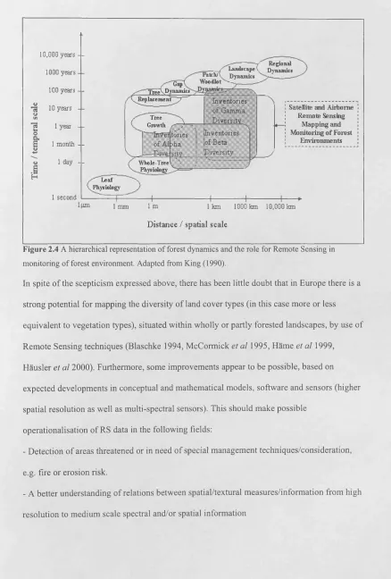
Figure 2.4 A hierarchical representation of forest dynamics and the role for Remote Sensing in monitoring of forest environment...60
Figure 2.5 Conceptual model of how fragmentation is related to habitat loss...74
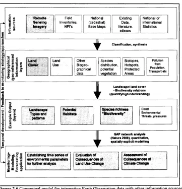
Figure 2.6 Conceptual model for integration Earth Observation data with other information sources for environmental monitoring in a habitat based approach...80
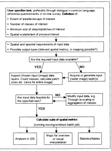
Figure 2.7 Proposed schedule for landscape analysis using EO and spatial metrics... 82
Figure 3.1 Aggregation of pixels from synthetic forest-non-forest image... 84
Figure 3.2 Extraction of edge (count) data from binary (forest-non-forest) images... 86
Figure 3.3 Location o f the test areas, shown on false colour WiFS im age...88
Figure 3.4 Geo-rectified subset of the Landsat TM scene... 89
Figure 3.5 Synthesised forest mask, pixel size 12.5 m, after edge detection... 91
Figure 3.7 Patch density in synthetic forest map plotted against forest cover... 93
Figure 3.8 Pixel size influence on Matheron index values...93
Figure 3.9 SqP as function o f pixel size and forest cover for synthetic images... 94
Figure 3.10 PPU as function of pixel size and forest cover...94
Figure 3.11 M values as function o f pixel size and forest cover for synthetic image... 96
Figure 3.12 M values as function of pixel size and number of patches for synthetic image ... 96
Figure 3.13 Scatter graph for Landsat TM band 3 and 4 ... 98
Figure 3.14 Scatter graph for WiFS band 1 and 2...99
Figure 3.15 Forest -non forest masks from classified images...99
Figure 3.16 Spatial configuration o f the values o f the Matheron index... 100
Figure 3.17 Comparison of metrics values between data sources... 101
Figure 3.18. Forest cover in windows with forest cover >0... 101
Figure 3.19 Metrics derived from WiFS data plotted against metrics derived from TM data 103 Figure 3.20 Spatial metric maps displayed together as different ‘channels’ in a false colour image...103
Figure 4.1 The selected subset... 113
Figure 4.2 FMERS forest map for area of interest, with NUTS-level 2 regions...114
Figure 4.3 Subsets o f CLC and FMERS maps located in Umbria and Toscana...115
Figure 4.4 CLC image for the area of interest, after re-classification to forest map... 116
Figure 4.5 Cross-tabulated image from CORINE and FMERS forest m asks...119
Figure 4.6 Digital Elevation Model of Italy...121
Figure 4.7 Example o f how maps o f forest presence are combined for masking in extraction of statistical parameters... 126
Figure 4.8 Moving windows concepts with and without overlap... 127
Figure 4.9 Simplified flowchart showing how results presented below are derived...128
Figure 4.10 Land cover ’’richness”, i.e. count of different land cover types... 134
Figure 4.11 Metrics ‘response curves’ or scalograms... 134
Figure 4.12 Average values of the SqP metric for the two data types plotted against window size in pixels resp. m eters... 136
Figure 4.13 Avg. patch density plotted against window size, CLC and FM ER S... 138
Figure 4.14 Avg patch density plotted against the avg. forest cover...138
Figure 4.15 Background patch count applied as possible fragmentation metric... 139
Figure 4.16 Standard deviation of the values in output cells, CLC data... 140
Figure 4.17 Standard deviation of the values in output cells, FMERS data...140
Figure 4.18 Local variability of CLC data... 141
Figure 4.19 Local variability of FMERS forest map data... 142
Figure 4.20 Local variability of spatial metrics from CLC data, expressed with Moran’s 1 . 142 Figure 4.21 Local variability of spatial metrics from FMERS with Moran’s 1...143
Figure 4.22 Plots of different metrics values from the same data source, 2400*2400 m w indow s...148
Figure 4.23 Plots of different metrics values from the same data source, 19200*19200 m windows...151
Figure 4.24 R-square, expressing agreement between metrics values from CLC and FMERS data... 154
Figure 4.25 R-square-plot, window size transformed logarithmically...155
Figure 4.26 Forest cover and SHDI in 1200*1200 m cells from CLC forest m a p ... 158
Figure 4.27 CLC data with high-order catchment polygons...158
Figure 4.28 Examples of landscape metrics values reported at catchment level... 160
Figure 4.29 SHDI and Matheron metrics, extracted from CLC data to catchments...163
Figure 4.30 SHDI and Matheron metrics extracted from FMERS data to catchments 165 Figure 4.31 SHDI and Matheron metrics from CLC data, administrative regions...168
Figure 4.32 SHDI and Matheron metrics from FMERS data, regions...169
Figure 4.34 CLC and FMERS inputs compared for creation of FC-profiles of selected
administrative (NUTS-level 2) regions... 172
Figure 5.1 Land use in Vendsyssel around the year 1800... 190
Figure 5.2 Subset with Denmark from CLC map, base-map area m arked... 191
Figure 5.3 Geomorphological map of Vendsyssel... 193
Figure 5.4 Legends for land use - land cover data used in this study... 200
Figure 5.5 Subset of 5*5 km from image data sets used in this chapter...201
Figure 5.6 Tentative re-classifications into thematic levels... 206
Figure 5.7 Test block 1 to 3 as KMS traffic maps and AAK LUC m a p s...216
Figure 5.8 Matheron index and Edge Density maximum values... 220
Figure 5.9 Average elevation and slope based on values in 25m cells, averaged to 1km cells for comparison and correlation with spatial metrics values...224
Figure 5.10 Example o f the ‘processing chain’ from Land Use to Hemeroby map... 228
Figure 5.11 8*7 km subset of TB1 at the landscape thematic level, AAK images with the grain sizes used in this study - plus the corresponding subset from the C L C ... 229
Figure 5.12 Scaling behaviour of the rasterised AAK data set in the test blocks...234
Figure 5.13 Scalograms for the number o f matrix/background patches in test blocks 237 Figure 5.14 1.5*2.5 km subset from the northern part o f Test Block 1 ... 237
Figure 5.15 Scaling effects of changing grain size for the Matheron index., AAK d ata 238 Figure 5.16 Two different approaches to depicting the scale dependence o f the SqP metric.239 Figure 5.17 Example of pair-wise comparison of metrics maps from the different sources. 247 Figure 5.18 Output (5km) cell-by-cell plots of patch count metrics values between the landscape thematic level and the forest and nature levels for AAK and LCP data...249
Figure 5.19 Output (5km) cell-by-cell plots of patch count metrics values between nature and forest thematic levels and between landscape and forest thematic levels, AAK data 249 Figure 5.20 Changing relation between the Matheron index for forest and for nature thematic layers with increased window size...250
Figure 5.21 Scatter-plots of selected relations between terrain features and structural metrics for the forest theme from the AAK map in 1km windows...254
Figure 5.22 Scatter graphs of combination of the NP and SHDI metrics values in geomorphological strata for AAK and LCP data, nature thematic le v e l...256
Figure 5.23 Relationship between Hemeroby values derived from AAK and CLC as scatter plots...258
Figure 5.24 Combined histograms o f Hemeroby values distribution for AAK and CLC data for window sizes from 1 to 5 k m ...265
Figure 5.25 Approaches to creating Hemeroby maps of the study a r e a ... 266
Figure 5.26 "Hemeroby map" o f Denmark based on CLC data... 267
Figure 6.1 Creation o f dwellings/floor space density surface with 25m grain size... 279
Figure 6.2 Local effects o f different theoretical afforestation scenarios around Hjorring 283 Figure 6.3 Summary o f effects on spatial metrics from different afforestation scenarios 287 Figure 6.4 Changes in Hemeroby index values (averages within 1*1 km windows) with the different scenarios...289
0.4 List of tables
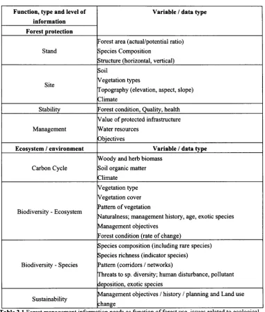
Table 2.1 Forest management information needs as function of forest u se ...28
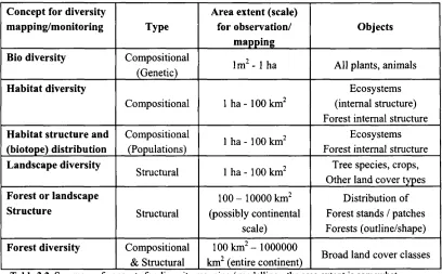
Table 2.2. Summary of concepts for diversity mapping / modelling...35
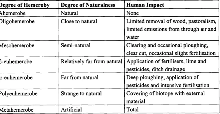
Table 2.3 Levels of Hemeroby for description and evaluation of biotopes...39
Table 2.4 Working concept for forest diversity assessm ent...56
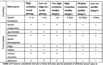
Table 2.5 Features considered relevant to forest diversity and the potential of different sensor types to monitor th e m ... 58
Table 3.1 Satellite data used for forest mapping... 88
Table 3.2 Correlation of the SqP metric derived from different pixel siz e s... 95
Table 3.3 Correlation of the PPU metric derived from different pixel siz e s... 95
Table 3.4 Correlation between M derived at varying pixel sizes... 97
Table 3.5 Correlations between initial forest area and the three spatial metrics from synthetic images at resolutions corresponding to imagery from the TM and WiFS sensors...97
Table 4.1 Matching CORINE and FMERS forest cover classes for the current study... 116
Table 4.2 Distribution of land cover classes in the two data sets... 117
Table 4.3 Co-occurrence o f pixel values in FMERS and CORINE land cover m aps...118
Table 4.4 Theoretical values of PPU and PPUN for varying window sizes and number of patches...124
Table 4.5 Patch count values from different window siz e s... 137
Table 4.6 Critical R values for varying number of observations with a = 0 .0 5 ...144
Table 4.7 Correlation coefficients between metrics, CLC 12*12 pixels window... 145
Table 4.8 Correlation coefficients between metrics, FMERS 6*6 pixels window...145
Table 4.9 Correlation coefficients between metrics, CLC 24*24 pixels window... 147
Table 4.10 Correlation coefficients between metrics, FMERS 12*12 pixels w indow 147 Table 4.11 Correlation coefficients between metrics, CLC 48*48 pixels window... 149
Table 4.12 Correlation coefficients between metrics, FMERS 24*24 pixels w indow 149 Table 4.13 Correlation coefficients between metrics, CLC 96*96 pixels window... 149
Table 4.14 Correlation coefficients between metrics, FMERS 48*48 pixels w indow 150 Table 4.15 Correlation coefficients between metrics, CLC 192*192 pixels window 150 Table 4.16 Correlation coefficients between metrics, FMERS 96*96 pixels window 151 Table 4.17 Summary of correlation coefficients between cover proportion and metrics values at increasing window sizes for CORINE land cover data... 152
Table 4.18 Summary of correlation coefficients between cover proportion and metrics values at increasing window sizes for FMERS forest map...152
Table 4.19 Agreement between metric values from different image sources at varying window sizes... 154
Table 4.20 Agreement between the two data sources on number of "background patches”. 156 Table 4.21 Summary at catchment level of spatial metrics from the CLC map, with medium window size 4800m ... 162
Table 4.22 Summary at catchment level of spatial metrics from the FMERS map, with medium window size 4800m ... 164
Table 4.23 The hierarchical approach illustrated...166
Table 4.24 Summary at administrative region level of spatial metrics from the CLC map, window size 4800m ... 167
Table 4.25 Summary at administrative region level of spatial metrics from the FMERS map, window size 4800m ...168
Table 4.26 Comparison of forest proportion values and derived diversity metrics from the input data for two administrative regions... 170
Table 4.27 FC values for catchments in Northern Italy for window size 1200m... 171
Table 4.29 Correlation coefficients for agreement between CLC and FMERS based values of the SHDI diversity index at different window sizes for selected geographic areas... 173 Table 4.30 Correlation coefficients for agreement between values o f the Matheron index, based on CLC and FMERS data, at different window sizes, selected geographic areas 175 Table 4.31 Mean values o f coefficients of variation for selected metrics from the CLC data and elevation from DTM... 176 Table 4.32 Mean values of coefficients of variation for selected metrics from the FMERS data and elevation from D TM ... 176 Table 4.33 Spearman’s rank correlation coefficients for agreement between spatial metrics from CLC and FMERS forest maps, for 12 administrative regions in Italy...178 Table 4.34 Spearman’s rank correlation coefficients for agreement between spatial metrics from CLC and FMERS forest maps, for 13 selected 4th level catchments... 178
Table 5.1 Proportion of forest land cover types from different mapping sources...205 Table 5.2 Relative area of non-matrix and non-background classes... 206 Table 5.3 Aggregation o f Land Cover Map (LCM) and Land Cover Plus (LCP) image data for landscape analysis at varying thematic resolutions...208 Table 5.4 Step-wise re-classification of land use data from the A A K ... 209 Table 5.5 Step-wise re-classification of land use classes from the CLC...211 Table 5.6 Kappa index of agreement for forest-non forest and nature-non nature images derived from the datasets at 25m grain size...212 Table 5.7 Percentage of land use types in the three test blocks, collected from 5m grain images with the “landscape” thematic resolution as described above... 217 Table 5.8 Metrics used in this chapter, categorised according to type... 219 Table 5.9 Hemeroby types with estimated NDP values and corresponding AAK classes .... 226 Table 5.10 Hemeroby types with estimated NDP values and corresponding CLC level 3 classes... 226 Table 5.11 Proposed assignment of rough Hemeroby classes to output from averaging 227 Table 5.12 Total count o f separate patches o f selected classes with different responses to image grain size (scaling behaviour)... 231 Table 5.13 Cover proportions and average patch size in hectares for Test Block 1 ... 232 Table 5.14 Diversity metrics values expressed as SHDI for the entire test b lo ck ...235 Table 5.15 Diversity metrics values expressed as SHDI for the entire test block, only
Table 5.28 Spatial metrics from AAK, Nature theme values by (dominant) geomorphologic type in 1 km windows... 255 Table 5.29 Spatial metrics from LCP, Nature theme values by (dominant) geomorphologic type in 1 km windows... 255 Table 5.30 Values o f integrated Hemeroby index from AAK and CLC data respectively.... 258 Table 5.31 Correlations between output cell values of Hemeroby and the suite o f spatial metrics for AAK land use data...260 Table 5.32 Correlations between output cell values of Hemeroby and the suite of spatial metrics for CLC land use data... 262
Table 6.1 Definition of soil types and colour codes for the soil classification o f Denm ark.. 278 Table 6.2 Cross-tabulation of test image with forest types assigned according to pixel ranking by FTI against actual forest map from AAK at 25m ... 282 Table 6.3 Observed values of changes in metrics values per 1 * 1 km window for the four different scenarios - compared with the current situation...285 Table 6.4 Changes in Hemeroby values following implementation o f different afforestation scenarios... 287
1 Introduction
The forests o f Europe constitute the habitats for a wealth of animals and plants - by definition
not least trees. At the same time, they form parts of cultural landscapes, or when of
appropriate size, they constitute landscapes in their own right. Most forests are also
production systems that provide timber and other products, as well as having important
recreational functions. There are thus many reasons to take interest in the way forests are
managed and their ecological state. Field-based forest mapping and inventories are however
expensive and time consuming, and not considered feasible for environmental monitoring
tasks. Therefore methods for rapid and inexpensive mapping and analysis o f forest have been
requested during the last centuries. At the same time, the discipline of landscape ecology has
emerged, providing a framework for spatial analysis and quantification of landscape structure.
Meanwhile the availability o f satellite images, starting with the successful launch of the
Landsat-1 satellite in 1972, offers synoptic views of landscapes and data in digital format that,
if interpreted correctly can be converted to maps of land cover and possibly land use. Today
several satellite platforms provide very-high-resolution imagery o f pixel size down to 60cm as
well as multi-spectral data well suited for discrimination of vegetation types. Following the
revolutionary development o f computers and their exponentially increasing power to perform
calculations, it has been possible to readily implement extraction o f the many metrics of
spatial structure, that has been proposed in the ecology and landscape ecology literature. The
intuitive observation, that spatial structure affects biological diversity and habitat quality,
supported by findings from island biogeography, has led to several attempts to statistically
link measures o f landscape structure and ground-survey based observations of flora and fauna,
accompanied by definition o f new metrics.
This specific study aimed at contributing to sustainable forest management and land use
land cover data, as well as satellite imagery that was processed to produce forest maps. The
objective o f this thesis was thus to select, and if necessary develop spatial metrics that can
be used to relate forest and landscape structure with the state of ecological systems at the
landscape level. It should be possible to derive the metrics through processing of satellite
imagery and from existing map data stored in Geographical Information Systems (GIS).
Several theoretical and empirical studies have shown that ecological processes are
hierarchically structured, as has also been found for landscape features. Values o f spatial
metrics appear to depend on the scale at which they are calculated, typically expressed by the
pixel size of the imagery from which the underlying maps are derived. It was therefore
considered important to assess the influence of scale on the selected metrics, and if possible to
quantify scaling effects in order to allow comparison of metrics values derived from different
data sources.
In the literature survey (chapter 2 o f this thesis), the complex relationship between spatial
structure and biological diversity and naturalness of landscapes is explored, with focus on
forest and woodlands. The concepts of scale in Remote Sensing, biology and landscape
ecology respectively were compared, and the issue of scaling addressed, especially relating to
influence o f scale on metrics values. The relation of metrics to dominating theories in
conservation biology and landscape ecology is discussed, as well as the possible use of Earth
Observation (EO) data and derived metrics in forest management. Fragmentation, seen as a
state as well as a process, is introduced as field of study o f special interest.
The theoretical considerations and practical approaches taken throughout the studies for this
thesis can be summarised in the following hypotheses:
Certain relationships can be found between biological diversity and naturalness (state)
Different properties of landscapes are/can be revealed from data at different spatial
and thematic resolutions.
The scaling behaviour of spatial metrics can be quantified and displayed graphically.
Combinations of spatial metrics can be optimised to yield information on forest and
landscape structure in order to characterise landscapes at local and regional levels.
The last three o f hypotheses above naturally lead to formulation o f various research questions,
posed in order to test different assumptions, these questions are stated in the empirical
chapters, which are structured as follows:
Chapter 3 describes the first empirical study, where focus was on metrics describing forest
structure, with the Umbria region in central Italy as the study area. Forest maps were made
from detailed GIS information and from high resolution (Landsat-TM sensor) and medium
resolution (IRS-WiFS scanner) satellite images. Scaling effects on metrics of fragmentation
were predicted from synthesised images degraded to increasingly coarser resolutions and
compared with metrics values from the EO based forest maps, and the possibility of
extrapolating values found at high resolution through use o f larger-area maps at lower
resolution was assessed.
In the subsequent study, described in chapter 4, the objective was to describe forest structure
and diversity over larger areas, with output as maps as well as tables and graphs. The spatial
extent increased to cover Central and Northern and Italy and surrounding areas. Existing land
use/land cover (LUC) data from the Corine Land Cover (CLC) database and a satellite based
forest map were used for comparison of metrics values over large areas, now including
metrics o f forest area, patch numbers and diversity. A Moving-Windows (M-W) method for
extraction of metrics values in areas of similar extent was implemented, allowing output of
results as thematic maps o f metrics values, thus visualising spatial structure. Scalogram curves
were used to describe scaling effects. Results from M-W calculations were analysed at
hierarchical levels. A Forest Concentration (FC) profile metric was proposed, which allowed
multi-scale description of the distribution of forest within a region or study area (however any
object o f interest can be described).
Then, chapter 5 presents results from in a study that covered Vendsyssel, the northernmost
part o f Denmark. Here focus moved to application of spatial metrics for description of
landscape structure and diversity, particularly for assessment of naturalness and disturbance.
Spatial metrics derived from maps at different thematic levels were compared, with the
objective o f evaluating their sensitivity to changing spatial and thematic resolution. Input data
were vector and raster based LUC maps from the Area Information System (AIS). Changing
resolution was found to influence patch count metrics strongly and with an unpredictable
response to grain size; metrics o f fragmentation changed linearly with grain size and metrics
of cover area and diversity showed little change. Correlations between metrics values from
different data sources and thematic levels were found to change significantly with window
size employed in the M-W method. A spatial Hemeroby index was introduced and metrics
values from LUC data at 25m pixel size found to be highly correlated with values from CLC
data at 250m pixel size. This provided evidence in favour of creating large-area Hemeroby-
maps, based on CLC data.
The final empirical study is described in chapter 6. Here the objective was to demonstrate
possible applications of spatial metrics and M-W for forest and landscape management.
Different afforestation scenarios were created for Vendsyssel, a simple and fast method was
used for assignment of new forest types to selected target areas, and changes in metrics values
and FC profiles were calculated. Different responses to the simulated landscape changes were
observed, and change-maps as well as tables and FC-curves provided promising tools for
In the conclusion in chapter 7, a synthesis o f the findings from the empirical studies is made,
and recommendations are provided for quantification of fragmentation using EO data and
spatial metrics and on the use o f spatial metrics for environmental monitoring at landscape,
regional and national levels.
All references used are listed in chapter 8, and chapter 9 contains some more personal
comments regarding the process of preparing this thesis as well as acknowledgements. The
implementations o f moving-windows calculation of the spatial metrics, scaling and averaging
operations are documented in the IDL-scripts in Appendix 1, while Appendix 2 contains a list
2 Literature review
This chapter opens with a discussion of the terms criteria and indicator, using the meanings
attributed to them in the so-called Helsinki Process (Granholm et al 1996). Then other
approaches to the indicator concept are presented, such as the CIFOR definitions (Stork et al
1997). Direct assessment and quantification o f biodiversity is a large and complicated task,
which requires intensive fieldwork, often by researchers with specialised knowledge. It was
therefore considered outside the scope o f this and previous projects to devise methods for
quantifying on-the-ground biodiversity with values derived only from EO data. However, it
was found important to provide an overview o f how (and if) biological diversity can be
measured and quantified - and how precise and reliable the results are - in order to find the
extent to which the use o f remote sensing can contribute to or supplement conventional
(labour intensive) methods of environmental monitoring.
Spatial metrics derived from digital EO data are more valuable, and applicable for
(ecosystem/conservation) management purposes, when there are solid theoretical links
between the biological processes and properties o f land cover maps (Haines-Young and
Chopping 1997, McCormick and Folving 1998, Gustafson 1998). Thus a section o f the
literature review is devoted to outlining basic ecological theories with spatial aspects and
discussing how they relate to and incorporate statistical measures of diversity and of
landscape geometry. The nature of natural (forest) ecosystems, in that they are complex and
nested systems makes it relevant to look closer at scaling issues, as done in section 2.3.3. The
potential relationships between spatial metrics from land cover maps and results from
numerical modelling o f meta-populations in real and simplified landscapes are addressed, and
the use o f “neutral” models discussed, i.e. assessment of metrics values from artificially
generated ‘images’ of ideal landscape where the properties under investigation can be
controlled (Gardner and O ’Neill 1991, With and King 1997). This can help select a group of
Working with EO data poses some practical problems during the process of moving from raw
sensor data to reliable land cover or habitat maps. It is not within the scope of this thesis to
review the wide range of possible image processing techniques, to that end 'standard
approaches’ based on recommendations found in the literature will be used, and examples of
their implementation are shown in subsequent chapters.
2.1 Sustainability and Biodiversity in environmental policy
In this section, a summary will be made of how the concepts of criteria and indicators,
sustainability and biodiversity are defined and applied in environmental sciences, policy and
management.
2.1.1 The need for definitions
For the purpose of protection and planning of Europe's forests at inter-national and continental
level, a strong interest exists in getting a broad view o f their state, be it in terms o f vegetation
health, species composition or environmental conditions in general (Granholm et al 1996,
European Commission 1999, Duniker 2000). In particular, it has been considered worth
investigating the potential of Earth Observation and Geographical Information System (GIS)
techniques for characterising and monitoring forests and their stability as habitats (Scott et al
1993, Haines-Young and Chopping 1995, Jones 1998, Hansson 2000).
The spatial structure of forests, and knowledge of the processes that it reflects, can be used to
derive some of the criteria and indicators that are needed for monitoring o f forest
sustainability. Thus, one o f the intentions of this review is to examine and describe how the
spatial structure within forests influences biological diversity. This implies identifying
methods for (a quantitative) description o f the shape or outline the forest elements and their
position relative to other land-cover types (typically expressed in terms of connectivity and/or
be used as indicators of sustainable forest management or naturalness. It must be stressed
here, that these indicators are tools for the assessment of the sustainability of forest- and
landscape-management, their numerical values are not goals in themselves. Thus this review
will not go into detail with the precise definitions, but rather look at the link between what
should be indicated (level o f sustainability) and the available remote sensing based techniques
to monitor forested landscapes.
However before doing so, some definitions and concepts must be clarified. Standardised,
operational definitions are essential if different persons are to make similar measurements of
similar entities in order to be able to analyse and compare the results (Morrison and Hall
2002). What is for example meant by this much talked about “landscape level” at which we
aim to do our analyses? What do we understand by a “habitat” - perhaps the spatial
expression o f (the presence of) a niche - depending on the species? How are ecosystems
defined and delimited? What actually are “Core Areas” and “Hot Spots” - and to what degree
do these concepts depend on the context in which they are used? And finally, what do we
mean by words such as “criteria” and “indicator”? (ibid.) The following section provides some
material to address these questions.
2.1.2 Criteria and Indicators
The concepts o f Criteria and Indicators (C&I) are widely used, and their use as parts of
systems for environmental assessment is a special case of their general use - the specification
and/or selection o f C&I for specific uses, such as assessing the sustainability o f forestry being
far from simple or without conflicts (Stork et al 1997, Mosseler and Bowers 1998, Hansson
2000).
According to Stork et al (1997) a criterion is a standard that a thing is judged by. In the forest
context it can be seen as a state or aspect of the dynamic process o f the forest ecosystem, or a
principle of sustainable forest management (or well managed forest). The way criteria are
formulated should give rise to a verdict on the degree of compliance in an actual situation (van
Bueren and Blom, in Dobbertin 1998). In the framework of the ‘Montreal process’ (ref.
Section 2.1.3 ) a criterion is characterized by a set o f related indicators which are monitored
periodically to assess change (Granholm et al 1996) - thus a criterion can be seen as a
category of conditions or processes by which sustainable forest management may be assessed.
An indicator is a measurable attribute of a system component (Duinker 2000), that can
ultimately be expressed as a number, i.e. quantified. An indicator is a quantitative or
qualitative parameter, which can be assessed in relation to a criterion. It describes in an
objectively verifiable and unambiguous way features of the ecosystem or the related social
system, or it describes elements of prevailing policy and management conditions and human
driven processes indicative of the state of the eco- and social system (van Bueren and Blom,
in Dobbertin 1998).
In the Montreal Process (see section 2.1.3), an indicator is a measure (measurement) of an
aspect of the criterion, a quantitative or qualitative variable which can be measured or
described and which, when observed periodically, demonstrates trends (Granholm et al 1996).
In a CIFOR working paper, Stork et al (1997, Box 1, p.3), note that C&I form indispensable
parts of a hierarchy of assessment tools:
Principle: A fundamental truth or law as the basis o f reasoning or action.
Criterion: A standard that a thing is judged by.
Indicator: An indicator is any variable or component o f the forest ecosystem or the relevant
management systems used to infer attributes of the sustainability o f the resource and its
utilisation.
Verifier: Data or information that enhances the specificity or the ease o f assessment o f an
These definitions are good for theoretical considerations, but in disagreement with the
definitions given above following Duinker (2000). According to the CIFOR definitions, the
word ‘indicator’ is often used when it should rather be verifier, the border between these
concepts will in practice be hard to define. A review of the different meanings o f criteria and
indicators can also be found in Granholm et al (1996, report 1). Accepting the definitions in
the Helsinki process o f a criterion, as something describing the different sides of
sustainability on a conceptual level (Ministry of Agriculture and Forestry 1994), the goal of
developing criteria is clearly outside the scope o f this thesis - which will instead look more
into how indicators can be defined or selected and calculated. This is in line with the Helsinki
process definition of indicators as typically quantitative measures of change. Thus an
important criterion for selecting an indicator based on EO data is that it is sensitive to
environmental changes as manifested in spatial structure at the landscape level.
2.1.3 Sustainability - the concept applied to forestry
The definitions found indicate a close relationship with management, which is reasonable, as
the concept of sustainability generally refers to processes and (land use) practices. Following
the resolutions from the Ministerial Conference on the protection o f forests in Europe,
Helsinki, June 1993 (Finnish Ministry of Agriculture and Forestry 1993): "sustainable
management means the stewardship and use o f forests andforest lands in a way, and at a
rate, that maintains their biodiversity, productivity, regeneration capacity, vitality and their
potential to fulfil, now and in the future, relevant ecological, economical and social functions,
at local, national and global levels, that does not cause damage to other ecosystems The
last part indicates the awareness that no part of the landscape can be monitored in isolation.
Just as we can not ignore the forested parts when examining agricultural landscapes, we can
not leave out the surrounding “matrix” consisting of land used for agricultural, urban or other
purposes, when we examine the structure o f forests in order to monitor their environmental
status, for nature protection and conservation purposes. Meanwhile, we can not leave out the
practical or even aesthetic motives (Haines-Young and Chopping 1996). Thus, criteria for
sustainable forest management should not only focus on maintaining production capacity, nor
on the actual biological diversity, but also on the structure and dynamics o f forest in relation
to the surrounding landscape and the people that inhabit it. This point o f view is reflected in
the six criteria agreed upon at European ministerial level through the decisions o f the
ministers at the Helsinki meeting (Finnish Ministry of Agriculture and Forestry 1993). The
criteria for sustainable forest management are:
1. Maintenance and appropriate enhancement of forest resources and their
contribution to global carbon cycles;
2. Maintenance of forest ecosystem health and vitality;
3. Maintenance and encouragement of productive functions of forests (wood and
non-wood);
4. Maintenance, conservation and appropriate enhancement of biological
diversity in forest ecosystems;
5. Maintenance and appropriate enhancement of protective functions in forest
management (notably soil and water);
6. Maintenance of other socio-economic functions and conditions.
The follow up on these decisions and the reporting from the countries is are often referred to
as ‘the Helsinki Process’. A ‘liaison unit’, since 2004 situated in Warsaw (before that in
Vienna), manages service to the member countries and the exchange of information, and
amongst other activities information is shared at the web site: http://www.mcpfe.org/.
Worldwide, several established international initiatives to develop criteria and indicators for
sustainable forest management (the Montreal Process, Helsinki Process, the International
Tropical Timber Organization (ITTO) Process) are now reaching an implementation stage
(United Nations 1998). The Montreal process is concerned with the temperate and boreal
forests outside Europe, and thus includes North America and Australia. The Tapparo protocol
management, while the ITTO has produced guidelines on sustainable management of tropical
forests (Granholm et al 1996, United Nations 1998). According to the Subsidiary Body on
Scientific, Technical and Technological Advice to the Convention on Biological diversity
(UNEP 1997, annex III), C&I provide a conceptual framework for forest policy formulation
and evaluation. Criteria define the essential elements of SFM while Indicators provide a basis
for assessing actual forest conditions. C&I, when combined with national goals are also useful
for assessing progress towards SFM and they can play an important role in defining the goals
of national forest programmes and policies.
2.1.4 Biodiversity - definitions and assessment
According to the convention o f biological diversity (CBD 1992): "Biological diversity means
the variability among living organisms from all sources including, inter alia, terrestrial,
marine and other aquatic ecosystems and the ecological complexes o f which they are part;
this includes diversity within species, between species and o f ecosystems. ”
2.1.4.1 The value o f biodiversity
The economic value of biological diversity and possible future benefits, for instance in the
medical field, is being recognised, along with the realisation that the more diverse an
ecosystem is, the better equipped it is to withstand and recover from disturbance. In a strategy
paper from the European Commission (European Commission 1998, p. 1), the importance of
biological diversity is outlined as: “Biological diversity (biodiversity) is essential to maintain
life on earth and has important social, economic, scientific, educational, cultural,
recreational and aesthetic values. In addition to its intrinsic value biodiversity determines our
resilience to changing circumstances. Without adequate biodiversity, events such as climate
change and pest infestations are more likely to have catastrophic effects. It is essential fo r
maintaining the long term viability o f agriculture and fisheries fo r fo o d production.
production o f new medicines. Finally, biodiversity often provides solutions to existing
problems o f pollution and disease. ”
With the growing awareness at global and continental political decision making level
(internationally and within large countries such as USA, Canada, Brazil and Australia) it is
becoming clear that the relation between sustainable development and the maintenance of
biological diversity is becoming increasingly important, as well as the growing awareness of
the interactions between ecosystem composition, structure and functioning (EWGRB 1998,
part A, chapter 1). In the proceedings from the first expert meeting o f the European network
for forest ecology (EFERN), Oswald (1996) states that: “The conservation o f ‘biodiversity’ is
considered today as a major and integrated part o f sustainable forest management. But, as
biodiversity can concern different levels o f appreciation, i.e. populations, individuals and
/
VV7
genetic processes
demographic processes, life histories
interspecific fiteratction, ecosystem process
y
disturbances, land-use trends.
[image:25.466.39.408.46.394.2]FUNCTIONAL
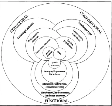
Figure 2.1. Compositional, structural and functional biodiversity, after Noss (1990).
2.1.4.2 Types o f biodiversity
It has become a widespread practice to define biodiversity in terms of genes, species and
ecosystems, corresponding to three fundamental and hierarchically-related levels of biological
organisation (WCMC 1995). In the context o f this discussion focus will be placed not so
much on the species diversity, but more on the ecosystem ‘domain’ when it overlaps
(spatially) with concepts such as habitat and landscape.
Hierarchy theory shows that higher levels of organisation incorporate and constrain the
behaviour o f lower levels (King 1990, Marceau 1999). Thus, knowledge o f structures and
processes dominant at one level - coinciding with a certain spatial scale - will allow us to
infer the processes that can take place and which species that will ‘fit in’ at lower levels or
utilised by McGarigal and McComb (1995) and by Rolstad et al (2000) in a study of
woodpeckers in a mosaic of forests and cultivated land. In a report on ecological conditions of
old-growth.Douglas-fir forests in the North-western United States, Franklin et al (1981,
referred in Noss (1990)) distinguished between compositional, structural and functional
biodiversity, as illustrated in Figure 2.1, see also Table 2.4, page 56. This approach has since
been applied intensively in ecological research, where ‘function’ sometimes is replaced by
‘development’, indicating that this is the component of biodiversity with the strongest
temporal dependence, or sensitivity to temporal scale when it comes to observation of
parameters. For a recent review o f concepts, terms and applications, see Puumalainen (2001).
2.1.4.3 Spatial levels of biodiversity
Whittaker (1972) defined and discussed a selection of diversity metrics. He introduced the
measures o f Alpha, Beta and Gamma diversity, to be used along with the concepts of niche
and hyperspace (of niches). The definitions below are taken from Gale (1996), but are
commonly accepted.
Alpha diversity is the variety o f the organisms that occur in a particular place or habitat, this is
often also called the ‘local diversity’.
Beta diversity is defined as
a) The diversity between or among more than one community or along an environmental
gradient, or
b) The variety o f organisms within a region arising from turnover o f species among habitats.
Beta diversity can thus be considered the change rate of the Gamma diversity, which is the
Landscape-level or regional diversity. Clearly what should be aimed at and focused on, when
investigating the applications o f remote sensing techniques, is whether and how it is possible
define some links between the Gamma diversity and the spatial structure of forests and
The terms Epsilon and Delta diversities are used to respectively denote inventory or area
diversities and gradients o f Alpha and Gamma diversity across regions and continents (Stoms
and Estes 1993), thus making comparisons possible on a global scale. The concepts are
illustrated in Figure 2.2.
1 I n v e n t o r y d i v e r s i t i e s '
Epsilon I regional
sampling unit: 1-100 mio ha
Gam m a/ landscape
sampling unit: 1000-1 mio ha
Alpha / within community
sampling units 0.1 to 1000 ha
P oin t/ micro habitat
sampling units 0.0001 to 0 01 ha
D i f f e r e n t i a t i o n d i v e r s i t i e s
Delta / geographic gradients;
Sampling units Alpha in same community type
Domain: landscape to region
Beta / environmental gradients;
Sampling units Alpha in different communities,
Domain: community to landscape
Pattern / micro gradients;
Sampling units Points in same community,
[image:27.483.8.476.34.514.2]Doman pant to community
Figure 2.2 Levels o f biological diversity as defined by W hittaker (1972). The m aps sketches to the left
represent inventory levels o f richness; those on the right show differentiation levels or changes in
com position across gradients. Sam pling unit sizes indicate approxim ate spatial dim ension for each
ecological scale
2.1.4.4 Demands for indicators of biodiversity
At the European level a project was initiated by the European Environment Agency (EEA) to
define criteria and indicators of forest diversity. The object of the BEAR project is to
“fo rm u la te an integrated system o f indicators o ffo re st biodiversity that are applicable over a
wide range o f European biogeographic regions, an d at regional, landscape an d stand levels.
(Hansson 1998, p. 2). It is further stated (ibid. p. 4) that ideally an indicator should be:
• able to differentiate between natural cycles/trends and those induced by anthropogenic
stress,
• capable of providing continuous assessments over a wide range o f stress,
• sufficiently sensitive to provide an early warning of changes,
• distributed over a broad geographical area, or otherwise widely applicable,
• easy and cost-effective to measure, collect, assay and/or calculate.
The work done in this project is presented in Larsson et al (2000) and partly at the project web
site: http://www.algonet.se/~bear/. Among the main achievements o f the project was the
agreement on a common scheme o f key factors of biodiversity applicable to European forests.
These factors are divided into structural, compositional and functional factors. There are
different factors for the structural (physical characteristics) and compositional (biological
component) types at different spatial scales while the functional key factors, which relate to
natural disturbances and human influence are the same across the scales (Larsson et al 2000,
chapter 3.1). The main recommendations from the project are as follows:
1) to introduce the key factor approach in monitoring of forest biodiversity, and
2) to make a further division into different ‘forest types for biodiversity
assessment’ in the reporting of the key factors (in all 33 different forest types
were identified, they mostly correspond to the national classification
schemes), and finally
3) to standardise indicators, methodology and protocols.
2.2 Use of landscape ecology concepts in forest and landscape
assessment and monitoring
This section is intended to provide conceptual links between the types of information needed
by forest managers at different levels and the tools provided by landscape ecology in terms of
understanding processes and identifying and quantifying patterns that are of relevance.
Important concepts in this context are habitat and habitat quality, structure and scale, which
2.2.1 Forest management information use and needs
Rural landscapes, o f which forest and woodland are important parts, need protection and
careful management. This is reflected in the principles outlined in the declarations from the
European ministerial conferences in Helsinki 1993 (Forest) and Sofia 1995 (The Pan-
European Biological and Landscape Diversity Strategy, PEBLDS (Smith and Gillet 2000))'.
Sustainable management includes preservation of the structural and biological diversity of the
agricultural and forested landscapes. In order to develop such management practices, an
understanding o f the landscapes spatial and temporal dynamics is needed, as stated by Stoms
and Estes (1993), Turner et al (1993), European commission (1999).
According to Kohl and Paivinen (1996), remote sensing has the potential to act as an
instrument to provide harmonised European forestry statistics. Lin and Paivinen (1999) list
five user groups for forest information:
International organisations, NGO’s and environmental organisations
National ministries
Research and academic institutes
Forest Industry
Forest owners
These groups obviously have different information needs, which are only to a certain degree
to be fulfilled using EO techniques, as illustrated in Lin and Paivinen (1999) and discussed by
Kohl and Paivinen (1996) - refer Table 2.1, see also Table 2.5, on page 58.
Function, type and level of information
Variable / data type
Forest protection
Stand
Forest area (actual/potential ratio) Species Composition
Structure (horizontal, vertical)
Site
Soil
Vegetation types
Topography (elevation, aspect, slope) Climate
Stability Forest condition, Quality, health
Management
Value of protected infrastructure Water resources
Objectives
Ecosystem / environment Variable / data type
Carbon Cycle
Woody and herb biomass Soil organic matter Climate
Biodiversity - Ecosystem
Vegetation type Vegetation cover Pattern of vegetation
Naturalness; management history, age, exotic species Management objectives
Forest condition (rate of change)
Biodiversity - Species
Species composition (including rare species) Species richness (indicator species)
Pattern (corridors / networks)
Threats to sp. diversity; human disturbance, pollutant deposition, exotic species
[image:30.462.35.417.65.515.2]Sustainability Management objectives / history / planning and Land use change
Table 2.1 Forest management information needs as function of forest use, issues related to ecological functions - from Lin and Paivinen (1999), based on Kennedy and Luxmoore (1994).
Forest owners and the wood/paper industry will typically have an interest in maintaining
resources for production, while environmental organisations and other NGO’s are concerned
with the biodiversity aspects. Thus, there is a challenge to define the correct level on which to
monitor forest conditions and ecosystem parameters. Often, much information can be found
Management Unit (FMU) level (Duinker 2000) - even if the size o f a typical FMU will vary
from country to country depending on tradition and geographical conditions.
A European Forest Information and Communication System (EFICS) has been proposed,
(McCormick el al 1995) in which EO data would have a central role and contribute to
monitoring and management of rural environment in general (Estreguil et al 2001, fig. 2).
This project currently continues as the European Forest Information System (EFIS)2. Different
NGO’s and parts of the forest industry have during the last decade been working on
developing various certification initiatives. These obviously need and do use some criteria for
sustainability (Baharuddin 1996). Such an ‘ecocertification’ procedure focuses on the quality
o f forest management and thus requires a prior definition of the criteria and indicators to be
used as a basis for the guarantees that buyers are expected to demand (Berthod 1998).
In Europe, ‘old growth forest’ is the closest we come to ‘natural’ forests, and special attention
is given to them, as it has become clear that they have a higher number o f species, many of
which can only live only under the special conditions found there, (Diamond 1988, Davis et al
1990, Spies 1998). The particular information needs o f such special forest types, that
typically serve as important habitat for specialised species were discussed as part o f the
BEAR project (Hansson 1998, Larsson et al 2000).
2.2.2 A biotope approach: Habitat quality
There is a knowledge gap - a lack o f precise ‘laws o f nature’ between the levels o f individual
organism behaviour (movement) and the one of spatial dynamics o f ecosystems that should be
protected (Karieva and Wennergren 1995, Mann and Plummer 1995). As ecosystems and their
dynamics per se can not be directly observed, they are either represented by some ‘indicator
species’ or substituted by features such as habitat, guild, vegetation type and disturbance and
guilds, which are then used to make possible assessments o f biological diversity and
naturalness. One promising approach is assessment of habitat quality, for which some
approaches are presented in this section.
In terrestrial environments, plants form a structured environment that provides the habitat for
the diversity of animal species (Franklin, 1995, May 1988). Forests are unique amongst
ecosystems in the degree to which a certain type o f vegetation, i.e., trees modify the
environment, and so to say define the available niches. It follows that in forests the habitat
quality or naturalness will vary according to management practices, ownership status and
history, as human intervention in forests normally consists of planting and removing trees of
certain species at certain times, often done in specific non-random spatial patterns (Franklin
and Forman 1987, Borgesa and Hoganson 2000).
It is beyond doubt that the biological diversity o f an area depends on environmental factors.
The most basic o f these are geological and climatic factors that follow geographic position
and topography (Nichols et al 1998, Griffiths et al 1999). Since trees are able to alter the local
microclimate, it follows that in forests and woodlands the diversity o f the fauna depends
strongly on the compositional, structural and developmental diversity of the vegetation
(McCormick and Folving 1998). This in turn altered by faunal activity ranging from insects,
harmful or just pollinating, to human settlement and forestry practices. Thus any
quantification or description of biological diversity in forested areas will, to some degree, be a
‘snapshot’ of many dynamic feedback processes, and only sustained monitoring can reveal the
dynamics and thus the functional diversity of the area. Another important factor determining
how many species a given patch of land, landscape or island can host is its area. The use and
reliability of area-species curves are described by e.g. May (1975) and later reviewed and
Diamond (1988) provides an interesting conceptual framework for assessing species diversity
with the QQID concept: resource Quality and Quantity, Interaction and Dynamic processes.
Quality is here to be understood as the habitat and resource factors that determine the ‘number
of niches’ or habitat diversity. Quantity represents the availability of area and productivity.
Interaction represents the complex issue o f species interactions, be it predation or plant
community successions, while finally D denotes the spatial dynamics including immigration,
extinction and in the long-term speciation. Roughly, Quality and Quantity correspond to the
structural and compositional aspects of biodiversity, while Interaction and Dynamics
correspond to the functional aspect. Stoms and Estes (1993), in a review o f what types of
biological diversity that can be monitored, and at what scales, argue for QQID as a useful
approach, although in practice the Structure-Composition-Function(Development) framework
is generally used. Wilson (1992, chapter 10, pp.171-199) mentions some factors of
importance for establishment and maintenance of biological diversity (species richness):
climatic stability, energy availability and area extent, and Griffiths et al (1999, table 1)
provide a list of factors thought to influence species richness, including habitat heterogeneity
(diversity/complexity) and disturbance, where moderate disturbance is seen as positive for
maintenance o f high biodiversity - as competitive exclusion is thus prevented. These factors
obviously have to be incorporated in sustainability assessment at landscape and regional
levels - perhaps more than has previously been done in biodiversity assessments. Along the
same lines, Angermeier and Karr (1994) recommend using the concept of ‘biological
integrity’ in environmental and conservation policy, in order to rethink prevailing views of
The EU-level report to the CBD (European Commission 1998) mentions that for
"Woodlands", there are several threats to biodiversity, amongst these are, listed by the sectors
from which they stem:
Agriculture: neglect o f small woodlands,
Forestry: Logging of old-growth forests, management intensification (and exotic species),
Transport and energy: fragmentation and acidification,
Tourism: forest fires,
i.e. largely threats that are eventually reflected in land cover changes, and thus can potentially
be monitored using earth observation and GIS techniques (Firbank et al 1996, Gallego et al
2000, Mucher et al 2000).
EE A has established a European-wide nature information system (EUNIS)3. A central part of
this system is habitat definition and classification, with the aim o f providing a common and
easily understood language for the description of all marine, freshwater and terrestrial habitats
throughout Europe (Davies and Moss 2002). The EUNIS definition o f habitat is “plant and
animal communities as the characterising elements of the biotic environment, together with
abiotic factors (soil, climate, water availability and quality, and others), operating together at a
particular scale.” For the purpose of categorising habitats sampling sizes ranging from lm 2 to
100m2 are found adequate, - at the smaller scale, still, microhabitats are found, at larger
spatial scales the EUNIS habitats can be grouped to “habitat complexes” - of which estuaries
are used as an example, but which also will be the case for many woodland types. The EUNIS
habitat classification system has been used for designation of NATURA 2000 sites (European
Commission 1999, Estreguil et al 2001, see also section 2.3.1.1). Thus, a prerequisite o f this
project is the ability to map relevant habitats types using RS data - at a spatial resolution that
requires high-resolution input imagery, refer section 2.3.2.