A note on the estimation of long run relationships in dependent cointegrated panels

Munich Personal RePEc Archive

A note on the estimation of long-run

relationships in dependent cointegrated

panels

Di Iorio, Francesca and Fachin, Stefano

Department of Statistical Sciences, University of Naples Federico II,

Faculty of Statistics, University of Rome ”La Sapienza”

1 September 2008

Online at

https://mpra.ub.uni-muenchen.de/12053/

A Note on the Estimation of Long-Run

Relationships in Dependent Cointegrated

Panels

Francesca Di Iorio1_{and Stefano Fachin}2

1 _{Department of Statistical Sciences, University of Naples Federico II}

v. L. Rodin´o, 80138 Naples, Italy,[email protected]

2 _{Faculty of Statistics, University of Rome ”La Sapienza”}

p.le A. Moro 5, 00138 Rome, Italy,[email protected]

Abstract. We address the issue of estimation and inference in dependent non-stationary panels of small cross-section dimensions. The main conclusion is that the best results are obtained applying bootstrap inference to single-equation estimators. SUR estimators perform badly, or are even unfeasible, when the time dimension is not very large compared to the cross-section dimension.

Keywords: Panel cointegration, FM-OLS, FM-SUR.

1

Introduction

The estimation of cointegrating relationships in heterogenous, dependent panels can be considered a still largely unsettled problem. Although efficient system methods are available (FIML by Groen and Kleibergen, 2003, DSUR by Mark, Ogaki and Sul, 2005, FM-SUR by Moon, 1999), they are all feasible only when (i) the number of time observations (T) is much larger than that of cross-section observations (N), and, (ii), there is no cointegration across units. Since both conditions are highly unlikely to hold two questions arise. First, is this really a problem from the empirical point of view? The second question stems from considering that efficiency improvements are desirable in order to have more accurate asymptotic interval estimates and tests. Since simulation inference applied to standard single-equation estimators has been shown to deliver good results (seee.g., Psaradakis, 2001, Chang, 2004, Fachin, 2007), do we really need to use a system estimator? The first aim of our paper is thus to compare the estimation performances of single-equation and system estimators in non-stationary panels with short-run dependence across units. Since FM-SUR (contrary to DSUR) is feasible in systems of the dimension typically encountered in practice, we will concentrate on this estimator and

⋆

2 Di Iorio, F. and Fachin, S.

its single-equation analogue, FM-OLS (Phillips and Hansen, 1990). Second, we will compare simulation and asymptotic inference performance of the FM-OLS estimator with those delivered by asymptotic inference on the FM-SUR estimator. We shall now first discuss the bootstrap inference procedures (sec-tion 2), then present the design and results of our Monte Carlo experiment (section 3), while some conclusions are drawn in section 4.

2

Bootstrap procedures

Consider for the sake of simplicity the case of two I(1) variables, Y and X, observed on a panel ofN units and T time observations. We assume a lin-ear long-run equilibrium relationship, with possibly heterogenous coefficients, holds in all units. Formally:

yit=θi+βix1it+uyit (1)

where xit = xit−1+uxit. In both cases i = 1, . . . , N, and t = 1, . . . , T.

Bootstrap inference involves two key steps: first, constructing the pseudo-datasets; second, defining the test statistics or confidence intervals to be used. Let us examine them in turn.

When constructing pseudo-data sets from non-stationary dependent pan-els the key point is to reproduce the presence of dependence both in the time series and in the cross-section dimensions. The former aspect has been the subject of the vast debate, whose details are beyond the scope of this paper (for a review, see Politis, 2003). As in Di Iorio and Fachin (2007), we will obtain the bootstrap noises applying the Stationary Bootstrap (SB; Politis and Romano, 1994) to the residuals of the FM regressions. To preserve the cross-unit dependence structure we simply need to resample the entireT×N

matrix of residuals. The systematic part of the bootstrap Data Generating Process (DGP) will depend on the purpose of the exercise: in the case of hypothesis testing it is the result of estimation under the null hypothesis to be tested, while for interval estimation of unconstrained estimation.

Summing up, when the aim is testing the hypothesis H0: βi = βi(0) the

bootstrap DGP is:

y∗

it=θbi+βi(0)x1it+u ∗y

it (2)

while for interval estimation we use

y∗

it=θbi+βbix1it+u ∗y

it (3)

whereαbi,βbi are the unconstrained FM-OLS estimates. In both casesbu ∗y it

is obtained applying a Stationary Bootstrap algorithm to the unconstrained residuals uby_it = yit −θbi −βbix1it. A thorough discussion of the choice of

p∗

=prop(|t∗

b|> t),witht=s −1

βi (βbi−β

(0)

i ), t ∗ b =s

∗−1

βi (βb

∗

ib−βbi),andβbandβbib∗

are the FM-OLS estimates ofβi computed respectively on the actual and on

theb−thboostrap pseudo-dataset (b= 1, . . . , B). Finally,sβi ands

∗

βi are the

estimated standard errors of these estimators. One simple way to compute confidence intervals is to take the desired quantiles (Q)of the distribution of the βb∗′

ibs. An α-level confidence interval for βi is then simply given by

[Qα/2(βbi∗), Q1−α/2(βbi∗)], where βb ∗ i =

h b β∗

i1. . .βb

∗ iB

i

is the vector of estimates obtained from the B bootstrap datasets. In principle, basing the interval on a pivotal quantity should deliver better results. Psaradakis (2001) sug-gests the percentile-t interval [βbi−Q1−α/2(tb∗)sβi,βbi−Qα/2(t

∗

b)sβi], where

the Gaussian quantiles used in asymptotic inference are replaced by those of the bootstrap distribution (empirical estimate of the unknown small sample distribution of the studentized statistic). The superiority of the second type of interval depends entirely upon the quality of the estimates of the standard errors (see e.g., Kilian, 1999). Hence, in our study we shall compute both type of intervals.

3

Monte Carlo experiment

3.1 Design

Moon and Perron (2004) carried out a simulation study in a traditional seem-ingly unrelated equations set-up of small system size (at most 4 equations, with up to 300 observations), concluding that system estimators were overall superior to single-equation ones. However, in non-stationary panel analysis the number of equations (units) is typically larger and that of time observa-tions smaller. For instance, an international macroeconomic panel including data at annual frequency starting at the early 1970’s for the largest world or european economies will have 10-20 units and 30-40 time observations. Does Moon and Perron’s conclusion hold for this sort of systems as well? To shed some light on the issue we will run a simulation experiment based on the DGP by Moon (1999). As we will see, our conclusions will in fact be rather different from Moon and Perron’s. The details of the DGP are as follows. In each unit of the panel two right-hand sideI(1) variables (X1, X2)

and a left-hand side variable (Y) are linked by a linear long-run equilibrium relationship:

yit=θi+β1ix1it+β2ix2it+uyit, i= 1, . . . , N; (4)

xkit =xkit−1+uxkit, k= 1,2; i= 1, . . . , N. (5)

The regression coefficients are generated as Uniform variates, respectively

θi ∼U nif orm(2,4) andβki∼U nif orm(1,3), wherek= 1,2.The errors of

4 Di Iorio, F. and Fachin, S.

units. More precisely, letting ux_t = [ux′

1tux ′

2t. . .ux ′ N t]

′

, where ux′

it = [ux1itux2it] ′

anduy_t = [uy_1tuy_2t. . . uy_{N t}]′

,we have

uy_t ux_t

(N+2N)×1

=M N 0 0 , R ∆ ∆′ Φ

(N+2N)×(N+2N)

,

whereRis a fullN×N matrix governing the dependence across units in the

uy′

its,∆is aN×2N matrix governing the dependence between theuxanduy

noises, and finally Φis a 2N ×2N matrix governing the dependence in the

ux′

swithin and across units. Since Moon and Perron report the performances of both FM-OLS and FM-SUR estimators to be negatively affected by the degree of endogeneity of theX’s, we decided to control accuratelyδ, impos-ing the homogeneity assumption. In our simulations we considered different values forδ, concluding that the relative performance of system and single-equation estimators does not seem to change with the degree of endogeneity. Here for space constraints we will thus report only results forδ= 0.4.The∆

matrix has a block form ensuring that there is constant correlation between the noise of any X and that of the relevant Y equation, and no correlation across units:

∆

N×2N =

    

δ δ0 0. . .0 0 0 0δ δ . . .0 0

..

. ... ... . .. ... 0 0 0 0. . . δ δ

    .

We instead allow heterogeneity across units in the dependence parameters, generating them asU nif orm(0.3,0.4) random variates; without loss of gen-erality we assume different X’s in the same unit to be orthogonal. Letting

φ(_lkij) =cov(ux

li, uxkj), the covariance between the noise ofXl in the ith unit

andXk in thejthunit, we then have:

Φ

2N×2N=

            

1 0 φ(12)₁₁ φ(12)₁₂ . . . φ₁₁(1N)φ(1₁₂N)

0 1 φ(12)₂₁ φ(12)₂₂ . . . φ₂₁(1N)φ(1₂₂N) φ₁₁(21) φ(21)₁₂ 1 0 . . . φ₁₁(2N)φ(2₁₂N) φ(21)21 φ

(21)

22 0 1 . . . φ (2N) 21 φ

(2N) 22

..

. ... ... ... . .. ... ...

φ(11N1)φ (N1) 12 φ

(N2) 11 φ

(N2)

12 . . . 1 0

φ(21N1)φ (N1) 22 φ

(N2) 21 φ

(N2)

22 . . . 0 1

            

The choice of the time and cross-section sample sizes have been fixed trying to strike a balance between empirical relevance, which suggests mediumN′

s

and smallT′

3.2 Results

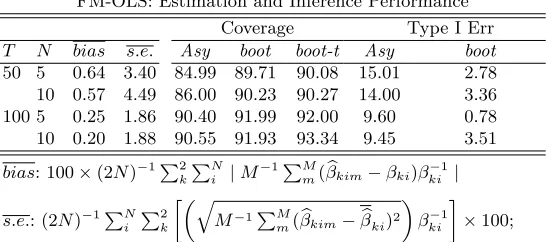
In Tables 1 and 2 we report summary statistics of the performances of re-spectively FM-OLS and FM-SUR estimators, further averaging over units and variables the usual Monte Carlo means.

Point estimation performance is evaluated by the average absolute relative bias 100×(2N)−1P2

k

PN i |M

−1PM

m(βbkim−βki)β −1

ki |while the dispersion

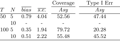
by the relative Monte Carlo standard error. The first remark in order is that the SUR procedure turned out to be practically unfeasible for T = 50 and

N = 10. The covariance matrix, although not exactly singular, was always so ill-conditioned that the estimators turned out to be highly numerically unstable even using a generalised Moore-Penrose inversion routine. Hence, we do not report them here.

Table 1

FM-OLS: Estimation and Inference Performance Coverage Type I Err T N bias s.e. Asy boot boot-t Asy boot

50 5 0.64 3.40 84.99 89.71 90.08 15.01 2.78 10 0.57 4.49 86.00 90.23 90.27 14.00 3.36 100 5 0.25 1.86 90.40 91.99 92.00 9.60 0.78 10 0.20 1.88 90.55 91.93 93.34 9.45 3.51 bias: 100×(2N)−1P2

k

PN i |M−

1PM

m(βbkim−βki)β−

1

ki |

s.e.: (2N)−1PN

i

P2

k

»„q

M−1P

M

m(βbkim−βbki)2

«

β−1

ki

– ×100; Coverage: proportion of 5% confidence intervals including the true value of the coefficient of interest;

6 Di Iorio, F. and Fachin, S.

other hand, the performance of asymptotic inference on the SUR estimator is simply disastrous, with Type I errors close to 50% whenT is not large with respect to N (that is, always for T = 50 and when N = 10 for T = 100) and around 20% even in the more favorable case of T = 100, N = 5. The reason for this extremely poor performance, not obvious from the bias and Monte Carlo variability statistics, is found in Table 3: the detailed results for the case T = 50, N = 5,δ = 0.41 _{show that the standard formulas for the}

variance of the SUR estimator grossly underestimate its actual variance.

Table 2

FM-SUR: Estimation and Inference Performance Coverage Type I Err T N bias s.e. Asy Asy

50 5 0.79 4.04 52.56 47.44

10 - - -

-100 5 0.35 1.94 79.72 20.28 10 0.51 2.22 55.48 45.52 -: not available (numerical overflow); all symbols and abbreviations: see Table 1

Table 3

Bias and Variability of FM-OLS and FM-SUR estimators T = 50,N= 5, δ= 0.4

bias M C s.e. σ_{b b}σ−M C s.e Unit OLS SUR OLS SUR OLS SUR OLS SUR

1 β₁ −0.13 0.44 5.1 5.3 3.8 2.2 1.2 3.1 β2 0.25 0.57 6.4 7.9 5.2 3.0 1.2 4.9

2 β1 −0.33 0.21 3.0 3.2 2.3 1.4 0.7 1.9

β₂ 1.09 1.27 6.0 6.6 4.7 2.7 1.4 3.9 3 β₁ 0.65 0.60 10.7 13.6 8.1 4.3 2.6 9.3 β2 −0.38 0.35 5.7 6.8 4.3 2.3 1.4 4.5

4 β1 0.52 2.34 9.8 12.7 8.2 4.5 1.6 8.2

β2 −0.38 0.01 3.8 4.4 3.1 1.8 0.8 2.7

5 β1 2.35 0.96 11.1 13.5 8.5 4.6 2.6 9.0

β2 0.23 1.10 4.7 5.3 3.6 2.1 1.1 3.2

MCs.e.: Monte Carlo s.e.;bσ: average estimated standard error×100; other symbols and details: see Table 1.

4

Conclusions

Our main conclusion is very simple: on the basis of our simulation exercise the best option in non-stationary panel analysis seems to be given by

single-1 _{Detailed results for the other cases do not provide any additional insights and}

equation estimators with bootstrap inference. The potential efficiency gains of SUR-type estimators remain such even in the restrictive case of no long-run relationships across units. In fact, when the time dimension is not very large relatively to the cross-section dimension the covariance matrix is likely to be so ill-conditioned to make the resulting estimates essentially meaningless. Further, even when some meaningful point estimates can be obtained, their variance is likely to be grossly underestimated by standard formulas, with disastrous effects on inference. These conclusions are in stark contrast to Moon and Perron’s (2004). However, this should not come as a surprise. The properties of SUR estimators depend critically upon the quality of the estimate of the covariance matrix. Obtaining good estimates may be an easy task in small systems, such as those examined by Moon and Perron, but may became very difficult in even slightly larger systems, such those considered in our study.

References

Chang Y. (2004): Bootstrap Unit Root Tests in Panels with Cross-Sectional De-pendency.Journal of Econometrics 120, 263-293.

Di Iorio, F. and S. Fachin (2007): Testing for breaks in cointegrated panels. Eco-nomics - The Open-Access, Open-Assessment E-Journal 2007-14.

Fachin, S. (2007): Long-Run Trends in Internal Migrations in Italy: a Study in Panel Cointegration with Dependent Units.Journal of Applied Econometrics 22, 401-428.

Groen, J. J. J. and Kleibergen, F. (2003): Likelihood-based cointegration analysis in panels of vector error-correction models.Journal of Business and Economic Statistics 21, 295-318.

Kilian, L. (1999): Finite-Sample Properties of Percentile and Percentile-t Bootstrap Confidence Intervals for Impulse Responses. The Review of Economics and Statistics 81, 652-660.

Mark, N.C., M. Ogaki and D. Sul (2005): Dynamic Seemingly Unrelated Cointe-grating Regressions.Review of Economic Studies 72, 797-820.

Moon, H.R. (1999): A note on fully-modified estimation of seemingly unrelated regressions models with integrated regressors.Economics Letters 65,25-31. Moon, H.R., Perron, B. (2004): Efficient Estimation of the Seemingly Unrelated

Re-gression Cointegration Model and Testing for Purchasing Power Parity. Econo-metric Reviews 23, 293-323.

Paparoditis, E., Politis, D.N., (2003): Residual-based block bootstrap for unit root testing.Econometrica 71, 813-855.

Phillips, P. C. B., Hansen, B. (1990): Statistical inference in instrumental regres-sions with I(1) processes.Review of Economic Studies, 57, 99125.

Politis, D.N., Romano, J.P. (1994): The Stationary Bootstrap.Journal of the Amer-ican Statistical Association 89,1303-1313.

Politis, D. (2003): The Impact of Bootstrap Methods on Time Series Analysis.

Statistical Science 18,219-230.