A New Approach of Solving Single Objective Unbalanced Assignment Problem

(1)

http://dx.doi.org/10.4236/ajor.2016.61011

A New Approach of Solving Single Objective

Unbalanced Assignment Problem

Ventepaka Yadaiah

1

_{, V. V. Haragopal}

2

1_{Department of Mathematics, Osmania University, Hyderabad, India} 2_{Department of Statistics, Osmania University, Hyderabad, India}

Received 9 December 2015; accepted 24 January 2016; published 29 January 2016

This work is licensed under the Creative Commons Attribution International License (CC BY). http://creativecommons.org/licenses/by/4.0/

Abstract

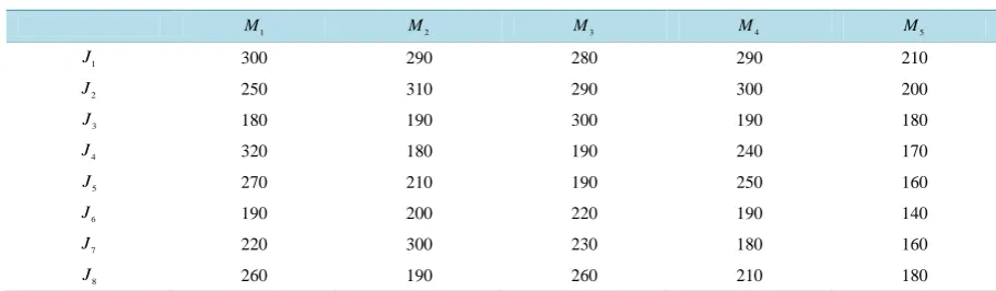
In this paper, we discuss a new approach for solving an unbalanced assignment problem. A Lexi- search algorithm is used to assign all the jobs to machines optimally. The results of new approach are compared with existing approaches, and this approach outperforms other methods. Finally, numerical example (Table 1) has been given to show the efficiency of the proposed methodology.

Keywords

Assignment Problem, Lexi-Search Algorithm, Jobs Clubbing Method

1. Introduction

Consider a problem which consists of a set of “n” machines M=

{

M M₁, ₂,M₃,,M_n

}

. A set of “m” jobs

{

1, 2, 3, , m

}

J= J J J  J which are to be considered assign for execution on “n” available machines. The execu-tion cost of each job on all the machines are known and menexecu-tioned in the matrix, namely assigned cost matrix (ACM) of order, where m>n. The unbalanced assignment problem is a special type of linear programming problem in which our objective is to assign number of salesmen to number of areas at a minimum cost (time). The mathematical formulation of the problem suggests that this is a 0 - 1 programming problem. It is highly de-generate all the algorithms developed to find optimal solution of transportation problem, applicable to unba-lanced assignment problem. However, due to its highly degeneracy nature a specially designed algorithm, wide-ly known as Hungarian method proposed by Kuhn [1], is used for its solution, and Kadhirvel and Balamurugan

[2] solved the unbalanced assignment problems using triangular fuzzy Numbers. Different methods have been presented for Assignment Problem and various articles have been published on the subject [3]-[7].

The objectives are to determine the optimal assignment cost, in such a way that all the jobs are to be allotted on the available machines in an optimum way. The mathematical formulation of the assignment problem [8] [9]

(2)

[image:2.595.83.539.97.230.2]

Table 1. Assigned cost matrix (ACM).

1

M M2 M3 M4 M5

1

J 300 290 280 290 210

2

J 250 310 290 300 200

3

J 180 190 300 190 180

4

J 320 180 190 240 170

5

J 270 210 190 250 160

6

J 190 200 220 190 140

7

J 220 300 230 180 160

8

J 260 190 260 210 180

2. Model Construction of Simple Assignment Problem

Minimize (Maximize):

1 1

m n

ij ij i i

Z C X

= =

=

∑∑

Subject to

1 1

n

ij j

X =

=

∑

; for i=1, 2, 3,,m

1

1 m

ij i

X

=

∑

; for j=1, 2, 3,,n

where 1, if the job is assigned to the machine. 0, if the job is not assigned to the machine.

th th

ij _th _th

i j

X

i j

 =  

Problem definition:

Also, if the numbers of jobs are not equal to number of machines, then it is known as an unbalanced assign-ment problem. Now consider the assumptions of choosing an unbalanced assignassign-ment problem as:

• The completion of a program from computational point of view means that the all jobs are assigned to vari-ous machines and final optimal assignment cost has been obtained.

• The number of jobs are more than number of machines.

The variants of assignment problem are considered by various researchers like Kagade & Bajaj [10] and Ava-nish Kumar [11]. From the work of these authors, they found that the approach of clubbing the costs of the jobs was implemented for multi objective problems and single objective problems, where as this paper considers the clubbing of jobs for an assignment problem by the exact solution problem with Lexi-search approach [12] [13].

3. Methodology

To determine the assignment cost as well as combination of job (s) Vs machine (s) of an unbalanced assignment problem for a set of “n” machines M =

{

M M₁, ₂,M₃,,Mn

}

. A set of “m” jobs J=

{

J J1, 2,J3,,Jm

}

which

are to be considered as assigned for execution on “n” available machines with an execution cost C_ij, where 1, 2, ,

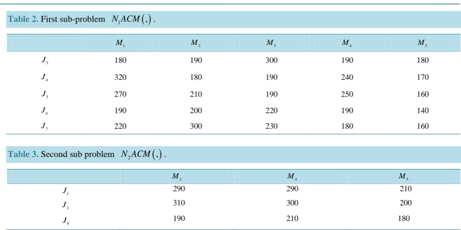
i=  m and j=1, 2,,n are mentioned in the ACM of order, where m > n. First of all, we obtain the sum of each row and each column of the ACM store and the results should be arranged in the array, namely,

(3)

[image:3.595.79.540.74.304.2]

Table 2. First sub-problem N ACM1

( )

, .

1

M M2 M3 M4 M5

3

J 180 190 300 190 180

4

J 320 180 190 240 170

5

J 270 210 190 250 160

6

J 190 200 220 190 140

7

J 220 300 230 180 160

Table 3. Second sub problem N ACM2

( )

, .

2

M M4 M5

1

J 290 290 210

2

J 310 300 200

8

J 190 210 180

defined assignment problem.Now we apply the Lexi-search approach to obtain the exact optimum solution of each sub problem (Tables 4-7). Finally, add the total assignment cost of each sub problem to obtain the optimal assignment cost along with assignment sets. And also we check the assignment cost for jobs clubbing problem (Table 8) through Lexi-search approach (Tables 9-11), getting the same value. To solve this problem we follow the following algorithm.

Algorithm

Step-1: Consider “m” jobs on “n” machines costs given as a matrix (ACM), which is an unbalanced assignment problem where

m

>

n

.

Step-2:

Step-2.1: Obtain the sum of each row and column of the ACM and the store the results in the arrays namely

Sum Row₋ and Sum Column₋ .

Step-2.2: Select the first m rows (jobs) on the basis of Sum Row− . That is, starting with the most minimum to next minimum to the array Sum Row− and deleting rows (jobs) corresponding to the remaining (m-n) jobs. Store the results in the new array that shall be the array for the first sub problem.

Step-2.2.1: If there is no remaining jobs, i.e., (m-n = 0), then go to step-3.

Step-2.2.2: If the remaining (m-n) jobs are still more than n, then repeat step-2.2 for the remaining jobs to form next sub-problem (s), else, step-2.3.

Step-2.3: If remaining jobs are less than n then deleting (n-m) columns (machines) on the basis of

Sum Column− . That is corresponding to value (s) most maximum to next maximum to form the last sub problem. Store the results in the new array that shall be the array for the last sub problem.

Step-3: If the total effectiveness of ACM is to be maximized, change the sign of each cost element in the ef-fectiveness matrix and go to step-4, otherwise go directly to step-5 if ACM has the total value as minimum.

Step-4: Arrange all the jobs J J J₁, ₂, ₃,,Jn according to their cost (i.e. available jobs). This arrangement

consists of n columns and m rows. Each column represents a machine, and the elements in that column are the costs arranged in increasing order according to their jobs.

Step-5: Include the job from the first machine in the partial solution value (psv) “w”. If the cost itself is greater than or equal to trial value (TRV) then stop. Otherwise go to next step.

Step-6: Calculate the bound.

Step-7: If the sum of bound and psv is greater than or equal to TRV then drop the job added in step 5, and go to step 5. Otherwise go to next step, i.e. go to Sub block (GS).

(4)

[image:4.595.88.539.52.726.2]

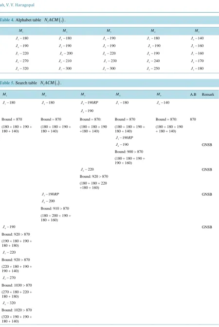
Table 4. Alphabet table N ACM1

( )

, .

1

M M2 M3 M4 M5

3 180

J − J4−180 J4−190 J7−180 J6−140

6 190

J − J3−190 J5−190 J3−190 J5−160

7 220

J − J6−200 J6−220 J6−190 J7−160

5 270

J − J5−210 J7−230 J4−240 J4−170

4 320

J − J7−300 J3−300 J5−250 J3−180

Table 5. Search table N ACM1

( )

, .

1

M M2 M3 M4 M5 A.B Remark

3 180

J − J4−180 J4−190RP J7−180 J6−140

5 190

J −

Bound = 870 Bound = 870 Bound = 870: Bound = 870 Bound = 870: 870

(180 + 180 + 190 + 180 + 140)

(180 + 180 + 190 +180 + 140)

(180 + 180 + 190 + 180 + 140)

3 190

J − RP

6 190

J − GNSB

Bound: 900 > 870

(180 + 180 + 190 + 190 + 160)

6 220

J − GNSB

Bound: 920 > 870

(180 + 180 + 220 +180 + 160)

3 190

J − RP GNSB

6 200

J −

Bound: 910 > 870

(180 + 200 + 190 + 180 + 160)

6 190

J − GNSB

Bound: 920 > 870

(190 + 180 + 190 + 180 + 180)

7 220

J −

Bound: 920 > 870

(220 + 180 + 190 + 190 + 140)

5 270

J −

Bound: 1030 > 870

(270 + 180 + 220 + 180 + 180)

4 320

J −

Bound: 1020 > 870

(5)

Table 6. Alphabet table N ACM2

( )

, .

2

M M4 M5

8 190

J − J8−210 J8−180

1 290

J − J1−290 J2−200

2 310

J − J2−300 J1−190

Table 7. Search table N ACM2

( )

, .

2

M M4 M5 A.B Remark

8 190

J − J8−210RP J8−180RP

Bound: 680 J1−290 J2−200 680

(190 + 290 + 200) Bound: 680 Bound: 680

(190 + 290 + 200) (190 + 290 + 200)

2 300

J −

Bound: 700 > 680 GNSB

(190 + 300 + 210)

1 290

J −

Bound: 700 > 680

(290 + 210 + 200)

2 310

J −

Bound: 730 > 680

(310 + 210 + 210)

Table 8. Jobs clubbing modified problem is N ACM3 ( ), .

1

M M2 M3 M4 M5

1 7

J ∗J 520 590 510 470 370

2 6

J ∗J 440 510 510 490 340

2

J 180 190 300 190 180

4 8

J ∗J 580 370 450 450 350

5

J 270 210 190 250 160

Table 9. Alphabet table N ACM3 ( ), .

1

M M2 M3 M4 M5

3 180

J − J3−190 J5−190 J3−190 J5−160

5 270

J − J5−210 J3−300 J5−250 J3−180

2 6 440

J ∗J − J4∗ −J8 370 J4∗ −J8 450 J4∗ −J8 450 J2∗J6−340

1 7 520

J∗J − J2∗J6−510 J1∗J7−510 J1∗J7−470 J4∗ −J8 350

4 8 580

(6)

[image:6.595.85.534.95.585.2]

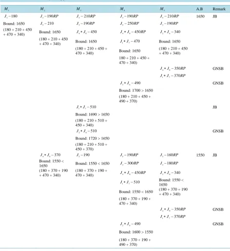
Table 10. Search table N ACM3 ( ), .

1

3 180

J − J3−190RP J5−210RP J3−190RP J5−210RP 1650 JB

Bound: 1650 J5−210 J3−190RP J5−250RP J3−190RP

(180 + 210 + 450

+ 470 + 340) Bound: 1650 J4∗ −J8 450 J4∗J8−450RP J2∗J6−340

(180 + 210 + 450

+ 470 + 340) Bound: 1650 J1∗J7−470 Bound: 1650

(180 + 210 + 450 +

470 + 340) Bound: 1650

(180 + 210 + 450 + 470 + 340) 180 + 210 + 450 +

470 + 340)

4 8 350

J ∗J − RP GNSB

1 7 370

J ∗J − RP

2 6 490

J ∗J − GNSB

Bound: 1700 > 1650 (180 + 210 + 450 + 490 + 370)

1 7 510

J∗J − JB

Bound: 1690 > 1650 (180 + 210 + 510 + 450 + 340)

2 6 510

J ∗J − GNSB

Bound: 1720 > 1650 (180 + 210 + 510 + 450 + 370)

4 8 370

J ∗ −J J5−190 J5−190RP J5−160RP 1550 JB

Bound: 1550 <

1650 Bound: 1550 < 1650 J3−300RP J3−180RP

(180 + 370 + 190 + 470 + 340)

(180 + 370 + 190 +

470 + 340) J4∗J8−450RP J2∗J6−340

1 7 510

J ∗J − Bound: 1550 <

1650

Bound: 1550 < 1650 (180 + 370 + 190 _{+ 470 + 340)}

(180 + 370 + 190 + 470 + 340)

4 8 350

J ∗J − RP GNSB

1 7 370

J ∗J − RP

2 6 490

J ∗J − GNSB

Bound: 1600 > 1550

(180 + 370 + 190 + 490 + 370)

Step-9: If partial solution value is greater than or equal to the TRV then drop the job added in step-8, and go to step-7. Otherwise go to step-10.

Step-10: If the sum of bound and psv is greater than or equal to TRV then drop the newly added job in step-8, and go to step -7.otherwise go to step 11.

Step-11: If the partial solution contains n − 1 jobs add the dummy job to the partial solution if it is greater than or equal to TRV then drop the dummy job and last two jobs from the partial solution. That is Jump out to the next higher order blocks (JO). If “w” contains only one job, go to step-5, otherwise go to step-8. Otherwise go to the next step.

Step-12: Now calculate the bound.

(7)

[image:7.595.77.539.108.519.2]

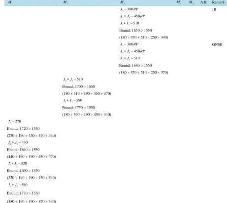
Table 11. Search table N ACM3 ( ), .

1

3 300

J − RP JB

4 8 450

J ∗J − RP

1 7 510

J ∗J −

Bound: 1650 > 1550

(180 + 370 + 510 + 250 + 340)

3 300

J − RP GNSB

4 8 450

J ∗J − RP

2 6 510

J ∗J −

Bound: 1680 > 1550

(180 + 370 + 510 + 250 + 370)

2 6 510

J ∗J −

Bound: 1700 > 1550

(180 + 510 + 190 + 450 + 370)

1 7 590

J ∗J −

Bound: 1750 > 1550

(180 + 590 + 190 + 450 + 340)

5 270

J −

Bound: 1720 > 1550

(270 + 190 + 450 + 470 + 340)

2 6 440

J ∗J −

Bound: 1640 > 1550

(440 + 190 + 190 + 450 + 370)

1 7 520

J ∗J −

Bound: 1690 > 1550

(520 + 190 + 190 + 450 + 340)

4 8 580

J ∗ −J

Bound: 1770 > 1550

(580 + 190 + 190 + 470 + 340)

Step-14: Include the latest possible job from the dummy job in“w”

Step-15: If psv is greater than or equal to TRV then drop the last dummy job and also the job from which the

th

i dummy job was assigned, and go to step-8. Otherwise go to next step.

Step-17: If sum of bound and psv is greater than or equal to TRV then drop the recently added job in “w” and go to step-14. Otherwise go to next step.

Step-18: Include the latest available job from the last job in “w”

Step-20: If the sum of bound and psv is greater than or equal to TRV then drop the latest job, and go to step- 18. Otherwise go to next step.

Step-21: If the number of elements in “w” is less than “n” go to step-18. Otherwise go to next step.

Step-22: Replace TRV by partial solution value and trial solution by w. Now go to step-18.

4. Illustration

(8)

costs are estimated as follows (in hundreds of rupees):

Solve the problem assuming that the objective is to minimize the total cost. Now obtain the sum of each row and column of ACM

( )

, , i.e., the sum of each row and each column is as follows:

1 2 3 4 5 6 7 8

1370 1350 1040 1100 1080 0940 1090 1100

J J J J J J J J

Sum Row₋ =

1 2 3 4 5

1990 1870 1960 1850 1400

M M M M M

Sum Column₋ =

We partition the matrix ACM

( )

, to define the first sub-problem N ACM₁

( )

, by selecting rows corresponding J J J J J₃, ₄, ₅, ₆, ₇ and second sub problem N ACM₂

( )

, by selecting rows corresponding to the jobs

1, 2, 8

J J J and by deleting columns corresponding to M M₁, ₃, then the modified matrices are as follows:

Sub-Problem-I:

N ACM

1

( )

,

Sub-Problem-II:

N ACM

2

( )

,

4.1. Now apply the Lexi-search method for Sub-Problem-I:

N ACM

1

( )

,

RP: Repitition, GNSB or JB: Go to next super block (JB), A.B or TRV = Absolute bound or Trail bound. The final optimal assignments of N ACM₁

( )

, as follows:

3 1

J →M , J₄→M₂, J₅→M₃, J₆ →M₅, J₇→M₄

4.2. Now Apply the Lexi-Search Method for Sub-Problem-II:

N ACM

2

( )

,

The final optimal assignments N ACM₂

( )

, is: J₁→M₄, J₂→M₅, J₈→M₂

The final optimal assignments assigned cost matrix (ACM) is : J₁→M₄, J₂→M₅, J₃→M₁,

4 2

J →M , J₅ →M₃, J₆ →M₅, J₇→M₄, J₈ →M₂. The Hungarian method gives us total assignment cost as 890 along with the other one job assigned to dummy machine, in other words the job that is assigned to dummy machine under the Hungarian method was ignored for further processing. While, the original problem was divided into two sub problems, which are balanced assignment problem in nature. Now for the two sub problems with the use of Lexi-search approach, the total cost 870 is recorded for the sub problem-I along with none of the jobs assigned to dummy machine, and the total cost 680 was recorded for the second sub problem-II along with none of the jobs assigned to dummy machine.Now the total cost of the assigned cost matrix (ACM) is 870 + 670 = 1550.

5. Job Clubbing Method

Jobs Clubbing Modified Problem Is

N ACM

3

( )

,

: Lexi-Search Approach

The final optimal assignments N ACM₃

( )

, as follows: J₃ →M₁, J₄∗J₈→M₂, J₅ →M₃, J₁∗J₇→M₄,

2 6 5

J ∗J →M

Total assignment cost = 1550.

Problem Hungarian method Lexi-search method

Unbalanced assignment problem Uses the dummy assignment Never uses the dummy assignment

Jobclubbing Gives optimum Gives exact optimum

6. Conclusion

(9)

va-ries from that of balanced assignment problems either in Hungarian method or Lexi-search approach. The only advantage is that the Lexi-search method gives an exact optimum value with the same time complexity. There-fore the present paper suggests a new approach of clubbing the jobs for solving the unbalanced assignment problem with Lexi-search methodology.

References

[1] Kuhn, H.W. (1955) The Hungarian Method for the Assignment Problem. Naval Research Logistic Quarterly, 2, 83-97. http://dx.doi.org/10.1002/nav.3800020109

[2] Kadhirvel, K. and Balamurugan, K. (2013) Method for Solving Unbalanced Assignment Problems Using Triangular Fuzzy Numbers. Journal of Engineering Research and Applications, 3, 359-363.

[3] Turkensteen, M., Ghosh, D., Goldengorin, B. and Sierksma, G. (2008) Tolerance-Based Branch and Bound Algorithm for the ATSP. European Journal of Operational Research, 189, 775-788. http://dx.doi.org/10.1016/j.ejor.2006.10.062

[4] Basirzadeh, H. (2012) Ones Assignment Method for Solving Assignment Problems. Applied Mathematical Sciences, 6, 2345-2355.

[5] Frank, A. (2004) On Kuhn’s Hungarian Method—A Tribute from Hungary. Wiley Inter Science, Published Online.

[6] Pentico, D.W. (2007) Assignment Problem: A Golden Anniversary Survey. European Journal of Operation Research, 176, 774-793. http://dx.doi.org/10.1016/j.ejor.2005.09.014

[7] Singh, S., Dubey, G.C. and Rajesh Shrivastava, R. (2012) A Comparative Analysis of Assignment Problem. IOSR

Journal of Engineering (IOSRJEN), 2, 1-15. http://dx.doi.org/10.9790/3021-02810115

[8] Gillett Billy, E. (2000) Introduction to Operations Research—A Computer Oriented Algorithm Approach.Tata Mc- Graw Hill, New Delhi.

[9] Taha, H.A. (1971) Operation Research: An Introduction.MacMillan Inc., New York.

[10] Kagade, K.L. and Bajaj, V.H. (2010) A New Approach to Solve Fuzzy Multi-Objective Unbalanced Assignment Prob-lem. International Journal of Agriculture Statistics, 6, 31-40.

[11] Kumar, A. (2006) A Modified Method for Solving the Unbalanced Assignment Problems. Journal of Applied

Mathe-matics and Computation, 176, 76-82. http://dx.doi.org/10.1016/j.amc.2005.09.056

[12] Pandit, S.N.N. (1963) Some Quantitative Combinatorial Search Problems. PhD Thesis, IIT, Khargpur.