A Method for Implementing Counterfactual Experiments in Models with Multiple Equilibria

Munich Personal RePEc Archive

A Method for Implementing

Counterfactual Experiments in Models

with Multiple Equilibria

Victor, Aguirregabiria

University of Toronto

10 October 2009

A Method for Implementing Counterfactual

Experiments in Models with Multiple Equilibria

Victor Aguirregabiria

University of Toronto

October 6, 2009

Abstract

This paper proposes a method for implementing counterfactual experiments in es-timated models that have multiple equilibria. The method assumes that the researcher does not know the equilibrium selection mechanism and wants to impose minimum restrictions on it. Our key assumption is that the equilibrium selection function does not jump discontinuously between equilibria as we change marginally the structural parameters of the model. Under this assumption, we show that, although the equi-librium selection function is unknown, the researcher can obtain an approximation of this function in a neighborhood of the estimated values of the structural parameters. Under the additional assumption that the counterfactual equilibrium is stable, this ap-proximation can be combined with iterations in the equilibrium mapping to obtain the exact counterfactual equilibrium. We illustrate the differences between our approach and other methods, such as the selection of a counterfactual equilibrium that is closer to the equilibrium in the data, and equilibrium mapping iterations using the equilibrium in the data as the initial value. We show that, in general, these alternative methods are not consistent with the assumption that the equilibrium selection mechanism is continuous with respect to the structural parameters.

Keywords: Structural models with multiple equilibria; Counterfactual experiments; Equilibrium selection.

1

Introduction

Multiplicity of equilibria is a prevalent feature in static and dynamic games and in general

equilibrium models. Models with multiple equilibria do not have a unique reduced form, and

this indeterminacy poses practical estimation problems. In the context of discrete games

with incomplete information, recent papers have proposed two-step and sequential estimators

that significantly simplify the estimation of these models (Aguirregabiria and Mira, 2007;

Bajari, Benkard and Levin, 2007; and Pesendorfer and Schmidt-Dengler, 2008). Nevertheless,

the indeterminacy problem associated with multiple equilibria still remains an issue when

the researcher wants to use the estimated model to predict the effects of counterfactual changes in the structural parameters. Although we can use the data to identify which of the

multiple equilibria is the one observed in the data, we do not know which equilibrium will be

selected in a counterfactual scenario. In some contexts, a possible approach for dealing with

this issue is to calculate all of the equilibria in the counterfactual scenario and then draw

conclusions that are robust to whatever equilibrium is selected. However, this approach is

of very limited applicability because the different equilibria typically provide ambiguous or even contradictory predictions for the effects we want to measure. Given that one of the most attractive features of structural models is the possibility of implementing counterfactual

experiments, this is a very important issue in structural econometrics. This issue is clearly

illustrated in the recent literature on empirical dynamic oligopoly games. Most applications

in this area either do not present counterfactual experiments (Collard-Wexler, 2006, and

Sweeting, 2007), or ignore the issue of multiple equilibria in the counterfactual model (Ryan,

2009, see footnote 32 in page 49; and Dunne et al, 2009, see pages 33-34).

This paper proposes a simple approach for dealing with multiple equilibria when

under-taking counterfactual experiments with an estimated model. Under the assumption that the

equilibrium selection mechanism, which is unknown to the researcher, is a smooth function of

the structural parameters, we show how to obtain a Taylor approximation of the

counterfac-tual equilibrium. More specifically, we show that, although the equilibrium selection function

is unknown, the Jacobian matrix of that function, evaluated at the estimated equilibrium,

As in any Taylor approximation, the approximation error has the same order of magnitude

as the distance between the factual and the counterfactual parameters. Therefore, this

approach can be inaccurate when the counterfactual experiment does not imply marginal

changes in the parameters. For these cases, we propose to combine the Taylor approximation

with iterations in the equilibrium mapping. The idea is that the Taylor approximation can

be far away from the counterfactual equilibrium but close enough to lie within the dominion

of attraction of that equilibrium.

We illustrate the differences between our approach and other methods, such as the se-lection of a counterfactual equilibrium that is closer to the equilibrium in the data, and

equilibrium mapping iterations using the equilibrium in the data as the initial value. In

gen-eral, these alternative methods are not consistent with the assumption that the equilibrium

selection mechanism is continuous with respect to the structural parameters.

2

Model

Lety _∈Y and x_∈X be two vectors of random variables with discrete and finite support.1

Let P0 ≡ {Pr(y|x) : (y,x) ∈ Y × X} be a vector with the probability distribution of y

conditional toxin the population under study. The structural model is a parametric family

of probability distributionsπ(y|x,θ), whereθ _∈Θis a vector ofK parameters, andΘ_⊂RK

is a compact set. LetΠ(θ)be the vector with the probability distribution ofyconditional to

x in the model for a valueθ of the structural parameters: i.e.,Π(θ)_≡{π(y|x,θ) : (y,x)_∈

Y ×X}. The probability distribution Π(θ) is implicitly defined as the solution of a fixed

point problem. LetΨ(θ,P)be afixed-point or equilibrium mapping fromΘ×[0,1]|X||Y|_into

[0,1]|X||Y| _{such that Ψ(θ,P)≡ {ψ(y|x,θ,P) : (y,x) ∈Y ×X}. The vector Π(θ) is afixed}

point ofΨ(θ, .), i.e.,Π(θ) = Ψ(θ,Π(θ)). However, for some values ofθ, the mappingΨ(θ, .)

can have more than onefixed point. That is, the model can have multiple equilibria for some

values of the structural parameters. We use Γ(θ) to denote the set of equilibria associated

with θ. We know that Π(θ)belongs to Γ(θ) but we do not make any additional assumption

1_{We describe our approach in the context of a class of models in which all the variables have a discrete}

andfinite support. This is convenient because we can use standard derivatives to construct Taylor approxi-mations. However, it is possible to extend this approach to models where variables have continuous support by using Banach spaces and Fréchet derivatives.

on how Π(θ) is selected within the set Γ(θ). This class of econometric models includes as

particular cases discrete models with social interactions (Brock and Durlauf, 2001), quantal

response games (McKelvey and Palfrey, 1995), and static and dynamic games of incomplete

information (Bajari et al., 2009, and Doraszelski and Satterthwaite, 2009), among others.

Let θ0 be the true value of θ in the population under study. The model establishes

that P0 = Π(θ0). Suppose that P0 and θ0 are point-identified given a random sample on

{y,x}. Let ˆθ0 and Pˆ0 be our consistent estimates of θ0 and P0, respectively. Let θ_∗ be

a value of the vector of structural parameters that is different to ˆθ0. We denote θ_∗ as the

vector of counterfactual values of the structural parameters. The researcher wants to obtain

the counterfactual equilibrium P_∗ associated with θ_∗, i.e., P_∗ = Π(θ_∗), and compare this

equilibrium with the one estimated from the data,Pˆ0. However, although the researcher can

calculate the set of equilibria Γ(θ_∗) (i.e., the set offixed points of the mapping Ψ(θ_∗, .)), he

does not know which of these equilibria is P_∗.

It is clear that we need additional information/structure to selectP_∗ from among the set

of equilibriaΓ(θ_∗). A possible approach might be to impose restrictions on the characteristics

of the equilibrium P_∗ (e.g., stability, symmetry, Pareto optimality, maximum payoffs for a certain player) that define a subset ofΓ(θ_∗)such that all the equilibria in that subset provide

similar predictions. That is, we may specify anequilibrium selection mechanism that selects

a single equilibrium, or a very reduced set of equilibria, in Γ(θ_∗). However, in most of

the applications, these restrictions may be difficult to justify. The researcher would want to have a method for implementing counterfactual experiments that does not require these

additional assumptions.2 _{In this paper, we consider that the researcher is not willing to}

impose these restrictions. We propose an approach that imposes minimum conditions on the

characteristics of the equilibrium P_∗. Assumptions 1 and 2 specify our restrictions on the model.

ASSUMPTION 1: Ψ is twice continuously differentiable in θ and P.

ASSUMPTION 2: The equilibrium selection mechanism is such that Π(θ) is a continuous

differentiable function within a convex subset of Θ that includes ˆθ0 and θ_∗.

2_{In fact, if these restrictions were plausible, the researcher would incorporate them into his model to}

Our approach is agnostic with respect to the equilibrium selection mechanism. We assume

that there is such a mechanism, that it is a function, and that it does not "jump" between

the possible equilibria when we move over the parameter space. However, we do not specify

any particular form for the equilibrium selection mechanismΠ(.).

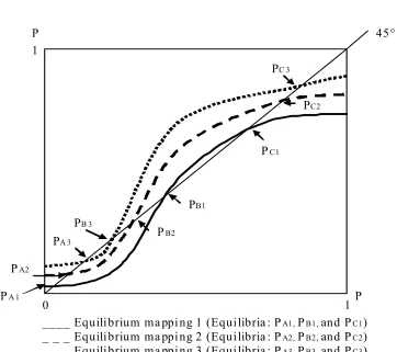
Figure 1 illustrates Assumption 2 for a simple model where P is a scalar. The three

curves represent the equilibrium mapping for three different values of the vector of structural parameters, say θ1,θ2, and θ3, such that ||θ2−θ1|| and||θ3−θ1|| are small, i.e., marginal

changes in the parameters. In thatfigure, an equilibrium is a value of Pfor which the curve meets with the 45-degree line, i.e., P = Ψ(θ,P). The set of equilibria associated with θ1

is Γ(θ1) ={PA1,PB1,PC1}. Suppose that Π(θ1) = PC1, i.e., when the vector of structural

parameters isθ1, the selected equilibrium is the one with the highest value ofP. Assumption

2 implies thatΠ(θ2) = PC2 andΠ(θ3) =PC3. That is, the equilibrium selection mechanism

does not jump discontinuously from the ’high-type’ equilibrium to the ’low-type’ (i.e., PA)

or to the ’middle-type’ (i.e., PB).3

Assumption 2 seems a reasonable condition when the researcher is interested in evaluating

the effects of a change in the structural parameters but keeping in the counterfactual the same equilibrium type as the one that generates the data.

3

Counterfactual experiments

We want to obtain the counterfactual equilibrium associated with θ_∗, that we denote P_∗.

Under Assumption 2, we know that Pˆ0 =Π(ˆθ0)and P_∗ =Π(θ_∗). Although Pˆ0,θˆ0, and θ_∗

are known to the researcher,P_∗ and the functionΠ(.)are unknown. Under Assumptions 1-2,

we can use afirst order Taylor expansion to obtain an approximation to the counterfactual

equilibriumΠ(θ∗)around the estimated vectorθˆ0. We do not know the functionΠ. However,

it is possible to use the equilibrium condition to obtain the Jacobian matrix ∂Π(ˆθ0)/∂θ0 in

terms of derivatives of the equilibrium mapping evaluated at (Pˆ0,ˆθ0). A Taylor expansion

3_{Some equilibrium ’types’ may disappear when we move along the parameter space. Therefore,}

As-sumption 2 establishes that the type of equilibrium Π(θˆ0) does not disappear when we move from ˆθ0 to θ_∗.

of Π(θ_∗)around ˆθ0 implies that:

Π(θ_∗) =Π(ˆθ0) +

∂Π(ˆθ0)

∂θ0 (θ∗−ˆθ0) +O(kθ∗−ˆθ0 k

2

) (1)

Note that Π(ˆθ0) = Pˆ0 that is known. Taking into account that Π(ˆθ0) = Ψ(ˆθ0,Π(ˆθ0)),

differentiating this expression with respect toθ, and solving for∂Π(θˆ0)/∂θ0, we can represent

this Jacobian matrix in terms of Jacobians of Ψ(θ,P) evaluated at the estimated values

(ˆθ0,Pˆ0). That is,

∂Π(θˆ0)

∂θ0 =

Ã

I₋ ∂Ψ( ˆ θ0,Pˆ0)

∂P0

!−1

∂Ψ(θˆ0,Pˆ0)

∂θ0 (2)

where Iis the identity matrix. Solving expression (2) into (1), we have that:

Π(θ_∗) =Pˆ0+

Ã

I₋ ∂Ψ(ˆθ0,Pˆ0)

∂P0

!−1

∂Ψ(ˆθ0,Pˆ0)

∂θ0 (θ∗−ˆθ0) +O(kθ∗−ˆθ0 k

2

) (3)

Therefore, when k θ∗ − θˆ0 k2 is small, the vector P˜_∗ ≡ Pˆ0 + (I− ∂Ψ(ˆθ0,Pˆ0)/∂P0)− 1

∂Ψ(ˆθ0,Pˆ0)/∂θ

0

(θ∗−ˆθ0)provides a good approximation to the true counterfactual

equilib-rium P_∗. Note that all the elements in the expression that describes P˜_∗ are known to the

researcher.

In some applications, the counterfactual experiments of interest are far from being

mar-ginal changes in the parameters. In such a situation, afirst order Taylor approximation could

be inaccurate. Higher-order approximations to Π(θ_∗) can be used. It is possible to show

that higher-order derivatives ofΠ(.)atˆθ0 depend only on derivatives ofΨat(θˆ0,Pˆ0), which

are known to the researcher. However, in applications where the dimension of the vector

P is large (e.g., dynamic games with heterogeneous players), the numerical computation of high-order derivatives of Ψ with respect to Pcan be computationally very demanding. An

alternative approach for improving the accuracy of the Taylor approximation is to combine

it with iterations in the equilibrium mapping. Suppose that P_∗ is an stable equilibrium.

This implies that there is a neighborhood of P_∗, say N, such that if we iterate in the

equi-librium mapping Ψ(θ_∗, .) starting with aP_∈N, then we converge toP_∗, i.e., if P1∈N and

Pk+1 = Ψ(θ_∗,Pk) for k ≥ 1, then limk_→∞Pk = P∗ (Judd, 1998, Theorem 5.4.2). The

attraction of P_∗. Then, by iterating in the equilibrium mapping Ψ(θ_∗, .) starting at P˜_∗ we

will obtain the counterfactual equilibriumP_∗.

It is important to explain the differences between the method that we propose here and two alternative methods for calculating a counterfactual equilibrium. The first alternative

method consists of iteration of the equilibrium mappingΨ(θ_∗, .)starting with the equilibrium

in the data. This approach will return the counterfactual equilibriumP_∗ if only if Pˆ0 belongs

to the dominion of attraction ofP_∗. It should be clear that this condition is stronger than the

one establishing that the Taylor approximation P˜_∗ belongs to the domination of attraction of P_∗.

A second alternative approach consists of calculating all the equilibria of the mapping

Ψ(θ_∗, .)and then selecting as the counterfactual the equilibrium with the smallest Euclidean

distance to Pˆ0. In general, this approach is not consistent with Assumption 2 which

estab-lishes that the equilibrium selection mechanism does not jump. We illustrate this issue in

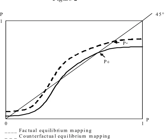
Figures 2 and 3. By Assumption 2, the counterfactual equilibrium P_∗ has the same type as

ˆ

P0. In Figures 2 and 3, P_∗ and Pˆ0 are ’high-type’ equilibria. In the example presented in

Figure 2, P_∗ is also the equilibrium in Γ(θ∗) that is closest (in Euclidean distance) to Pˆ0.

Therefore, our method and the "closest-equilibrium" method coincide in that case. However,

in Figure 3, the closest equilibrium toPˆ0 is notP_∗ but rather the ’middle-type’ equilibrium.

In this example, the "closest-equilibrium" method implies an equilibrium selection function

that is not continuous overhθˆ0,θ_∗i.

References

[1] Aguirregabiria, V. and P. Mira (2007): "Sequential estimation of dynamic discrete

games,"Econometrica, 75, 1—53.

[2] Bajari, P., L. Benkard and J. Levin (2007): "Estimating dynamic models of imperfect

competition," Econometrica, 75, 1331-1370.

[3] Bajari, P., H. Hong, J. Krainer, and D. Nekipelov (2009): "Estimating Static Models of Strategic Interactions,"Journal of Business and Economic Statistics. Forthcoming.

[4] Brock, W., and S. Durlauf (2001): “Discrete choice with social interactions”, Review of

Economics Studies, 68, 235-260.

[5] Collard-Wexler, A. (2006): "Demand Fluctuations and Plant Turnover in the

Ready-Mix Concrete Industry," manuscript. New York University.

[6] Doraszelski, U., and Satterthwaite, M. (2009): "Computable Markov-Perfect Industry

Dynamics," Manuscript. Department of Economics. Harvard University.

[7] Dunne, T., S. Klimek, M. Roberts, and Y. Xu (2009): "Entry, Exit and the

Determi-nants of Market Structure," NBER Working Paper 15313.

[8] Judd, K. (1998): "Numerical Methods in Economics," The MIT Press. Cambridge,

Massachusetts.

[9] McKelvey, R., and T. Palfrey (1995): "Quantal Response Equilibria for Normal Form

Games,"Games and Economic Behavior, 10, 6-38.

[10] Pesendorfer, M. and Schmidt-Dengler (2008): "Asymptotic Least Squares Estimators

for Dynamic Games," The Review of Economic Studies, 75, 901-928.

[11] Ryan, S. (2009): "The Costs of Environmental Regulation in a Concentrated Industry,"

Manuscript, MIT Department of Economics.

[12] Sweeting, A. (2007): ""Dynamic Product Repositioning in Differentiated Product In-dustries: The Case of Format Switching in the Commercial Radio Industry", NBER

Figure 1

PA 1 PA2

PA 3

PC 3

PC2

PC1

P P

0 1 1

45°

____ Equili brium ma ppi ng 1 (Equi libria : PA1, PB1, and PC1) _ _ _ Equili brium ma ppi ng 2 (Equi libria : PA2, PB2, and PC2) … … Equili brium ma ppi ng 3 (Equi libria : PA3, PB3, and PC3)

PB 3

PB2 PB1

Figure 2

P*

P0

P P

0 1 1

4 5 °

_ _ _ _ F a c tu a l e q u ili b ri u m m a p p i n g _ _ _ C o un t e r f a c t ua l e q u i lib r iu m m a p p in g P0 is t h e f a c t u a l e q u il ib r iu m

P* is t h e c o u n te r f a c tu a l e q u ili b r iu m

Figure 3

P*

P0

P P

0 1 1

4 5 °

_ _ _ _ F a c tu a l e q u ili b ri u m m a p p i n g _ _ _ C o un t e r f a c t ua l e q u i lib r iu m m a p p in g P0 is t h e f a c t u a l e q u il ib r iu m

P* is t h e c o u n te r f a c tu a l e q u ili b r iu m

Pclo s e st is th e e q u ili br i u m o f th e c o u n te r f a c tu a l m a p p i n g t h a t i s

c lo s e s t t o P0