Linear Programming for Optimum PID Controller Tuning

http://dx.doi.org/10.4236/am.2014.56084

Linear Programming for Optimum PID

Controller Tuning

Edimar J. Oliveira, Leonardo M. Honorio, Alexandre H. Anzai, Tamara X. Soares Federal University of Juiz de Fora, Juiz de Fora, Brazil

Email: [email protected], [email protected], [email protected],

[email protected]

Received 21 December 2013; revised 11 January 2014; accepted 18 January 2014

Copyright © 2014 by authors and Scientific Research Publishing Inc.

This work is licensed under the Creative Commons Attribution International License (CC BY).

http://creativecommons.org/licenses/by/4.0/

Abstract

This work presents a new methodology based on Linear Programming (LP) to tune Proportional- Integral-Derivative (PID) control parameters. From a specification of a desired output time do-main of the plant, a linear optimization system is proposed to adjust the PID controller leading the output signal to stable operation condition with minimum oscillations. The constraint set used in the optimization process is defined by using numerical integration approach. The generated opti-mization problem is convex and easily solved using an interior point algorithm. Results obtained using familiar plants from literature have shown that the proposed linear programming problem is very effective for tuning PID controllers.

Keywords

Linear Programming, Optimal Control, Interior Point Method, PID Tuning

1. Introduction

Since Dantzig invented the simplex method [1], the Linear Programming (PL) has been applied to solving prob- lems from many research areas. In 1984 Karmarkar presented interior point algorithm for solving linear pro- gramming [2] without the inconvenience of the exponential complexity of the Simplex algorithm.

programming is presented in [5] and reference [6] was pointed out the utilization of linear programming as one of the techniques to solve the unit commitment problem.

Proportional-Integral-Derivative (PID) controllers are a very efficient solution to obtain the desired output from the plant in steady state as well for dynamic response. Due to this aspect, the utilization of PID controllers has become very popular. The references [7] [8] present the main tuning methods utilized in academic research as well in industry. Two classical methods that are still utilized are the Ziegler-Nichols and the Cohen-Coon which utilize analytical approaches for analysis and tuning.

There are other analytical methods as described in [9]. Usually these methods employ heuristics [10] or intel- ligent methods like genetic algorithms [11], differential evolution [12] and particle swarm optimization [13]. These approaches demand the existence of a population according to an evolution criterion. Although these me- thods present good results, usually the computational time is high and requires several parameters tunings. One advantage of these methods is the fact that the objective function can be a heuristic rule that weights the output signal in various aspects at the same time.

However, despite of the fact that this characteristic is an advantage, the complexity of the objective function and the number of restrictions of the system increase the nonlinearity and the probability of the system is no convex. This characteristic can lead the population based optimization methods to have convergence problems [14] [15].

Seeking a faster and more efficient methodology for PID controller, this paper presents the development of a novel technique to tune the proportional-integral and derivative gains. As stated before, this device has been widely used as shown in many works encouraging the investigation of the possible improvements when it is tuned by using Linear Program (PL) based on interior point optimization, well known in several areas [16] [17] but still unexplored in the proposed area.

The main advantage of the proposed method resides on the fact that the systems designer can define the de- sired output in order to avoid saturations or other features and the optimization algorithm will return the appro- priate PID parameters values that minimize the error between the actual and the desired output. Manipulating the system to isolate the PID terms results in a linear optimization problem, with convex space solution, restricted and rapidly solved with the interior point optimization method.

This article is organized in the following manner: in Section 2 basic concepts of PID tuning are described; in Section 3 the methodologies employed are presented; in Section 4 the system model is shown and a detailed tu- torial example is presented to illustrate the methodology. At the end of Section 5 the results with an autonomous submarine are presented and in Section 6 some conclusions are presented.

2. Basic Concepts

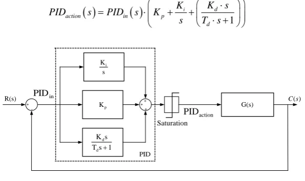
The standard system model considers the Plant G(s) and PID Controller structure as showed in Figure 1. In this figure C(s) represents the output response of the plant assuming a generic input R(s). The PID controller is composed by three terms whose transfer function is given by:

( )

( )

1

i d

action in p

d

K s

K

PID s PID s K

s T s

  ⋅ 

= ⋅_ + + _{⋅ +} _

 

  (1)

Figure 1.Standard system model.

+

-+ ++

+ G(s)

) (s C

Saturation

action

PID R(s) PIDin

PID s

Ki

p

K

1 s T

s K

d d

where PIDaction and PIDin represent respectively the output and input signals of the PID controller. The parame-

ters Kp, Ki and Kd are, respectively the proportional, integral and derivative gains. The time constant Td

repre-sents the derivative filters parameter to reduce a high frequency noise. In practices Td kd leading in this work

to adopt Td equal to 0.001.

Roughly speaking, the Kp term provides a proportional action to the input signal PIDin, the Ki term eliminate

the steady state error and the Kd term reduce the transitory oscillations.

Therefore when the controller gains are correctly tuned, the associated PID controller can provide good re- sults with linear and nonlinear systems considering small parameter variation. The dynamical and steady state performance requirements can be achieved through the specification of some criteria in time and frequency do- main, for example, the minimization of the quadratic error.

3. Proposed Methodology

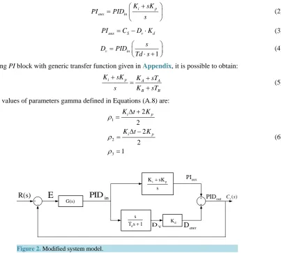
For the application of the proposed methodology, the standard representation of Figure 1 should be redrawn as shown in Figure 2 where the proportional and integral controllers were combined in a single block. In this dia- gram the signal (PIaux) represents the output of the proportional-integral block, (Dv) and (Daux) the output of the

derivative one. It is easy to verify that the output of the PID block (PIDout) is the sum of all control actions.

Considering that the output of the plant CS(t) is pre-specified by the designer face to a disturbance R(t) and

using numerical integration method as described in Appendix, it is possible to determine the PIDin(t) signal. It

can be seen from Figure 2 that PIDout(t) is equal to CS(t). So the problem is to determine the parameters of the

PID blocks to match the input PIDin(t) and output PIDout(t) signals.

Equations (2)-(4) describe the PID formulation in terms of parameters Kp, Ki, Kd and input/output signals

showed in Figure 2:

i p aux in K sK PI PID s +   = _{ }

  (2)

aux S v d

PI =C −D K⋅ (3)

1 v in s D PID Td s   = _{ } ⋅ +

  (4) Comparing PI block with generic transfer function given in Appendix, it is possible to obtain:

i p A A

B B

K sK K sT

s K sT

+ ₌ +

+ (5)

Then the values of parameters gamma defined in Equations (A.8) are:

1 2 3 2 2 2 2 1 i p i p

K t K

K t K

ρ ρ ρ ∆ + = ∆ − = = (6)

Figure 2.Modified system model.

+ -+

+

+ Cs(s)

R(s) aux D G(s)

E

Ki+ p

Therefore Equation (A.7) can be rewritten as follows:

( )

( )

(

)

(

)

aux in in aux

PI k =ρPID k +ρ PID k− +PI k− (7)

where k=2,3,,N. Considering Equations (3) into Equation (7) yields to:

( )

( )

( )

(

)

(

)

(

)

S v d in in S v d

C k −D k ⋅K =ρPID k +ρ PID k− +C k− −D k− ⋅K (8)

Rearranging (8), leading to Equation (9), as follows:

( )

( )

(

)

( )

v d in in S

D k K PID k ρ PID k ρ C k

∆ ⋅ + ⋅ + − ⋅ = ∆ (9)

where:

( )

( )

(

)

S S S

C k C k C k

∆ = − − (10)

( )

( )

(

)

v v v

D k D k D k

∆ = − − (11)

After obtaining all vectors of Equation (9), it is possible to calculate the parameters Kd, ρ1 and ρ2 by us- ing the linear programming formulation to take adjustable input and output signals. In this way, the optimization problem can be formulated as shown in Equations (12):

( )

( )

( )

( )

(

)

( )

( )

( )

1 2

2

1 2 1 2

1

2 1 2

Minimize

Subject to

1

0 50, 0 100

100 10, 0 ,

N

k

v d in in S

d

Te R k R k

D k K PID k PID k R k R k C k

K

R R ub

ρ ρ ρ ρ = = _ + _ ∆ ⋅ + ⋅ + − ⋅ + − = ∆ ≤ ≤ ≤ ≤ − ≤ ≤ ≤ ≤

∑

Te: Total error of the fitting from linear programming;

N: Number of equality constraints that is equal to the C(k) length; R1: Vector of right positive residue in the RN subspace;

R2: Vector of left positive residue in the RN subspace;

ub: Upper bound of residue variables. The ub equal to 200 is adopted in this paper. The rangers adopted for other variables have been enough to find the desire fitting.

Hence, considering an input and output signals with N values, it is possible to obtain a set of N-1 equations given by Equations (9) which is the set of constraints of the optimization problem (12). Nonetheless it is numer- ically unlikely that the equality constraints imposed by Equation (9) can be completely satisfied, thus the posi- tive residue variables R1(k) and R2(k) is added to provide enough slacks in the constraints. Then, the objective is to minimize the sum of these residues.

The compact form of problem (12) is written according to a linear optimization problem:

T min max Minimize Subject to c x Ax b

x x x

= ≤ ≤

(13)

where:

( ) ( ) ( 1;2( 1) 3)

2 1 3 2 1 3 1

, , , N N

N N N

x∈R − + c∈R − + b∈R − A∈R − − +

and 2(N 1)

U∈R − a vector with all elements equal to one. Thus:

( )

(

) ( )

(

)

[

]

[

]

( )

( )

T

1 1 2 2 1 2

T

1 , , 1 , 1 , , 1 , , ,

, 0, 0, 0 , with 1, ,1

2 , ,

d

x R R N R R N K

c U U

b C C N

The proposed LP problem (12) has spent low computational time because it has been written as a linear pro- gram and solved by using the ToolBox called linprog of MATLAB©based on a linear interior point solver [18], which is a variant of the Mehrotra’s predictor-corrector algorithm [19]. The advantage of using linear program- ming is related to a convex region close to a viable operating point. So, even under about one thousand linear constraints, the problem (12) spends about 3 seconds to find the solution.

Therefore, the solution of the LP problem (12) brings the values of the parameters Kd, ρ1 and ρ2 that better fit

the input/output signals to minimize R1(k) and R2(k). By replacing Kd, ρ1 and ρ2 in the set of Equation (6), it is

possible to calculate the values of Kp and Ki

4. Results

The results of the application of the proposed methodology will be presented in two parts, the first one dedicated to a tutorial case and the second one to tuning of an attitude control for vertical orientation of a vehicle in launching stage.

The time to complete the whole optimization process was only 3 sec in a MacBook pro core i5 with 4 Gb of RAM and the algorithm implemented in MATLAB© script program.

4.1. Tutorial Analysis

For this tutorial analysis it was chosen the plant from Equation (14) represented by its transfer function G(s) as described in reference [20].

( )

₍

₎₍

₎

1 5

G s

s s s

=

+ + (14)

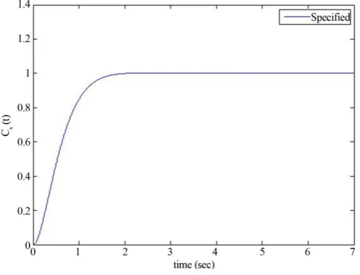
The specified output CS(t) in response to a unit step input R(t) can be seen in Figure 3. This curve was ob-

tained by using a standard second order model given by:

( )

n s

n n

C s

s ω

ζω ω

=

+ + (15) With ωn = 3, ζ = 1, Δt = 0.01 and time simulation equal to 7 seconds. It can be emphasize that the total ele-

ments of vector CS(t) is equal to N = 7/0.01 = 700 points.

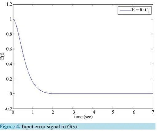
Considering the model presented in Figure 2, it is necessary to obtain all points of the curves utilized as coef- ficients in the composition of the optimization problem (12). Therefore, with a unit step R(t) and the specified Cs(t), the input signal E(t) to the plant transfer function G(s) is given by E(t) = R(t) − CS(t) whose curve is

shown inFigure 4.

Figure 4.Input error signal to G(s).

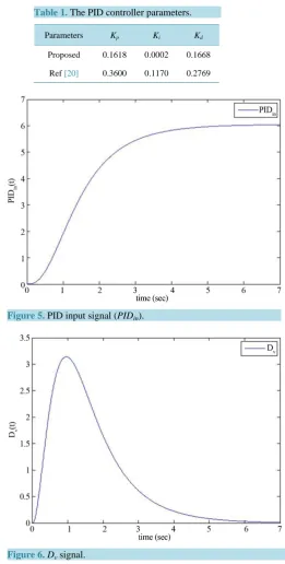
Figure 5 shows the input signal of PID controller (PIDin) that is obtained from E(t) as input signal of G(s) and

using trapezoidal integration showed in Appendix.

The last set of points needed to complete the coefficients of the problem (12) is Dv(t) obtained from PIDin by

using Equation (4) and trapezoidal integration. Figure 6 displays Dv(t) signal.

After all coefficients were calculated, it is possible to build the optimization problem (12) for the optimal PID parameter calculation. Using the LP Toolbox of Matlab Kd, ρ1 and ρ2 are obtained to match the input and output

signals with the total error of the fitting (Te) equal to 0.037. From Equations (6), it is possible to calculate the

values of Kp and Ki.Table 1 shows the best values of PID parameters obtained by the optimization process. In

addition, the second row of the table shows the PID proposed in reference [20].

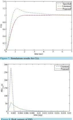
To evaluate the performance of the proposed methodology a simulation using the system of Figure 1 were carried out for both adjustable PID calculated from LP and PID of the literature [20]. Figure 7 presents these output results including CS(t). It can be observed that the methodology based on LP resulted in a best behavior

compared with literature. In addition, this figure shows that the C(t) followed the specified output being practi- cally identical to the desired one.

Figure 8presents the initial PIDaction related with the peak signal. This feature is important to avoid the action

control reaches the saturation limit. As seen in Figure 8, the maximum peak signal in the proposed LP approach is much lower than the corresponding peak displayed in literature [20]. Although it is not in the scope of this work, it is possible to modify the CS(t) in order to find other initial PIDaction.

4.2. Attitude Control

A basic flight of vehicle is composed by guidance, navigation and an attitude control systems [21]. The last one control system is responsible for vehicle vertical orientation. Usually, the utilization of conventional controller tuning techniques presents unsatisfactory performance due to plant characteristics. The proposed methodology will be applied to the PID design for the attitude control, in particular to maintain the vertical angle in respect with the vertical in 0˚. Thus this problem is similar to the control angle problem of the Inverted Pendulum Mod- el (IPM).

The linearized equation that represents the rotation movement of the shaft in respect with the center of gravity can be defined by:

(

)

m l⋅ ⋅ =θ M+m ⋅ ⋅ −g θ u (16) where θ is the relative shaft angle in respect with the vertical axe; l is the length of the shaft; M is the mass of the mobile support and is equal to 2 kg; m is the shaft mass and is equal to 0.1 kg; g is the acceleration of gravity, considered 9.81 m/s2; u represents the force produced by the PID control effort.

Table 1. The PID controller parameters.

Parameters Kp Ki Kd

Proposed 0.1618 0.0002 0.1668

Ref [20] 0.3600 0.1170 0.2769

Figure 5.PID input signal (PIDin).

Figure 6. Dvsignal.

model in frequency domain resulting in Equation (17). In a preliminary analysis it is possible to note that the re- sulting model is difficult to control due to the positive real part of one of the poles.

( )

( )

_{( )}

(

)

2 1

4.539

s G s

U s _s

Θ

= =

− (17)

In this case, since it is an inverted pendulum model (IPM), the system response must be fast and stable. Thus, the specified output signal CS(t) necessary to train the system is defined by the following parameter values ωn =

Figure 7.Simulations results for C(t).

Figure 8. Peak outputs of PIDaction.

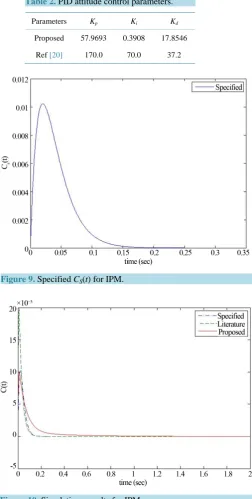
showed in Figure 9. In this case, the total elements of vector CS(t) is equal to N = 0.25/0.001 = 250 points. This

is the considerable amount of points in order to successfully complete the optimization process.

As seen in Figure 9, it must have a reduced time simulation for training control action to avoid the pendulum falls. Although there are strategies to automatically deal with this problem, it is out of the scope of this work. Therefore, the time simulation for training output signals is considered provided heuristically by the designer experience.

In Table 2 it is shown the both PID gain values by the proposed methodology and reference [20] for the in- verted pendulum model of the attitude control problem.

The performance of the proposed PID tuning is evaluated by using the system of Figure 1 where the time si- mulation of 2 sec was adopted. Figure 10 shows the output simulations of C(t) for proposed, literature and spe- cified. It can be observed that the LP approach presented the best behavior because the initial angle varies less than the PID adjusted from literature. It is important to mention that this feature results in less chance of the pendulum falling to or the control strategy just fails. In addition, the figure shows that the proposed PID tuning is capable to follow the specified output.

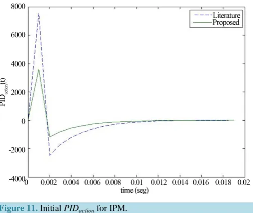
Figure 11 presents the initial PIDaction related with the peak signal. This feature is important to avoid the ac-

Table 2. PID attitude control parameters.

Parameters Kp Ki Kd

Proposed 57.9693 0.3908 17.8546

Ref [20] 170.0 70.0 37.2

Figure 9.Specified CS(t) for IPM.

Figure 10.Simulations results for IPM.

Analyzing the obtained results it is possible to observe that the optimized performance of the proposed con- troller was able to maintain the desired angular position for the projectile.

5. Conclusions

Figure 11.Initial PIDaction for IPM.

The method was described with the aid of a detailed tutorial analysis and a specific case of the attitude control of a flight vehicle was also analyzed obtaining excellent results. From the results obtained applying the proposed methodology the following aspects can be stressed out:

• The specified plant output can always be obtained close to the desired one with negligible error, if the system dynamics and saturation are considered.

• The obtained optimization problem is linear presenting a convex feasible region resulting in numerical ro- bustness.

• The computational time is small even with a large quantity of sample points for the training process.

• The proposed method can be modified to use nonlinear plant models once the curve construction processes are made outside the optimization stage.

• An extension of the methodology can be applied to adaptive control considering that the computational time is compatible with data acquisition time of the variables.

Acknowledgements

The authors would like to thank FAPEMIG, CAPES/PNPD and CNPq for the financial support.

References

[1] Dantzig, G.B. (1963) Linear Programming and Extensions. Princeton University, Princeton.

[2] Karmarkar, N. (1984) A New Polynomial Time Algorithm for Linear Programming. Combinatorica, 4, 373-395.

http://dx.doi.org/10.1007/BF02579150

[3] Delson, J.K. and Shahidehpour, S.M. (1992) Linear Programming Applications to Power System Economics, Planning and Operations. IEEE Transactions on Power Systems, 7, 1155-1163. http://dx.doi.org/10.1109/59.207329

[4] Chattopadhyay, B., Sachdev, M.S. and Sidhu, T.S. (1996) An On-Line Relay Coordination Algorithm for Adaptive Protection Using Linear Programming Technique. IEEE Transactions onPower Delivery, 11, 165-173.

http://dx.doi.org/10.1109/61.484013

[5] Boyd, S.P., Balakrishnan, V., Barratt, C.H., Khraishi, N.M., Li, X., Meyer, D.G. and Norman, S.A. (1988) A New CAD Method and Associated Architectures for Linear Controllers. IEEE Transactions on Automatic Control, 33, 268- 283. http://dx.doi.org/10.1109/9.404

[6] Padhy, N.P. (2004) Unit Commitment—A Bibliographical Survey. IEEE Transactions onPower Delivery, 19, 1196- 1205. http://dx.doi.org/10.1109/TPWRS.2003.821611

[7] Åström, K.J. and Hägglund, T. (2001) The Future of PID Control. Control Engineering Practice, 9, 1163-1175.

http://dx.doi.org/10.1016/S0967-0661(01)00062-4

ceedings on Control Theory and Applications, 149, 46-53.

[9] Toscano, R. and Lyonnet, P. (2010) A New Heuristic Approach for Non-Convex Optimization Problems. Information

Sciences, 180, 1955-1966. http://dx.doi.org/10.1016/j.ins.2009.12.028

[10] Ntogramatzidis, L. and Ferrante, A. (2011) Exact Tuning of PID Controllers in Control Feedback Design. Control

Theory and Applications, 5, 565-578. http://dx.doi.org/10.1049/iet-cta.2010.0239

[11] Alfaro-Cid, E., McGookin, E. and Murray-Smith, D. (2006) GA-Optimised PID and Pole Placement Real and Simu-lated Performance When Controlling the Dynamics of a Supply Ship. IEEE Proceedings on Control Theory and

Ap-plications, 153, 228-236.

[12] Zhao, S., Qu, B., Suganthan, P., Iruthayarajan, M. and Baskar, S. (2010) Multi-Objective Robust PID Controller Tun-ing UsTun-ing Multi-Objective Differential Evolution. IEEE 11th International Conference on Control Automation

Robot-ics & Vision (ICARCV), 2398-2403.

[13] Ren, Z., San, Y. and Chen, J. (2006) Improved Particle Swarm Optimization and Its Application Research in Tuning of PID Parameters. Journal of System Simulation, 18, 2870-2873.

[14] Honorio, L., da Silva, A., Barbosa, D. and Delboni, L. (2010) Solving Optimal Power Flow Problems Using a Prob-abilistic α-Constrained Evolutionary Approach. Generation, Transmission & Distribution, 4, 674-682.

http://dx.doi.org/10.1049/iet-gtd.2009.0208

[15] Leite da Silva, A., Rezende, L., Honório, L. and Manso, L. (2011) Performance Comparison of Metaheuristics to Solve the Multi-Stage Transmission Expansion Planning Problem. Generation, Transmission Distribution, 5, 360-367.

http://dx.doi.org/10.1049/iet-gtd.2010.0497

[16] de Oliveira, L., Carneiro Jr, S., de Oliveira, E., Pereira, J., Silva Jr., I. and Costa, J. (2010) Optimal Reconfiguration and Capacitor Allocation in Radial Distribution Systems for Energy Losses Minimization. International Journal of

Electrical Power & Energy Systems, 32, 840-848. http://dx.doi.org/10.1016/j.ijepes.2010.01.030

[17] de Souza, A., Honorio, L., Torres, G. and Lambert-Torres, G. (2004) Increasing the Loadability of Power Systems through Optimal-Local-Control Actions. IEEE Transactions on Power Systems, 19, 188-194.

[18] Zhang, Y. (1996) Solving Large-Scale Linear Programs by Interior-Point Methods under the Matlab Environment, Tech. rep., Department of Mathematics and Statistics, University of Maryland, Baltimore County, Baltimore.

[19] Mehrotra, S. (1992) On the Implementation of a Primal-Dual Interior Point Method. SIAM Journal on Optimization, 2, 575-601. http://dx.doi.org/10.1137/0802028

[20] Ogata, K. (1997) Modern Control Engineering Systems. 3rd Edition, Prentice Hall.

Appendix: Transfer Function Solution

This appendix presents the steps for the numerical integration process based on trapezoidal method. Therefore, a solution to a generic transfer function is presented in Equation (A.1) which is possible to represent a wide range of linear models for real plants. In this equation, X(s) represents the input signal and Y(s) is the output.

( )

( )

B B

K sT

Y s X s

K sT

+

= ⋅

+ (A.1)

Manipulating (A.1) and rearrange one yield:

( )

( )

( )

( )

B A A B

s⋅_T Y s −T X s _=K X s −K Y s (A.2)

In time domain Equation (A.2) becomes:

( )

( )

(

)

( )

( )

d

dt T y tB −T x tA =K x tA −K y tB (A.3)

or

( )

( )

(

)

(

( )

( )

)

d T y t_B −T x t_A = K x t_A −K y t_B dt (A.4)

Integrating both sides of (A.4) it is possible to obtain:

( )

( )

( )

( )

(

)

d d d

y t t x t t t t

B A A B

y t x t t

T y t T x t K x t K y t t

+∆ +∆ +∆

− = −

∫

∫

∫

Solving Equation (A.5) by using the trapezoidal integration method, leads to:

(

)

( )

(

)

( )

K t K t

T y t t T y t

K t K

T x t t T x t

∆ ∆  ₊  _{+ ∆ =} ₋          ∆  ₊  _{+ ∆ =} ₋          (A.6)

Simplifying Equation (A.6), it results:

(

)

(

)

( )

( )

y t+ ∆ =t ρx t+ ∆ +t ρ x t +ρ y t (A.7)

where: 1 2 3 2 2 2 2 2 2 A A B B A A B B B B B B

K t T

T K t

K t T

T K t

T K t

T K t

ρ ρ ρ ∆ + = + ∆ ∆ − = + ∆ − ∆ = + ∆ (A.8)

It can be observed that Δt represents the step of the numerical integration. In addition, it is important to em- phasized that the output signal y(t) can be obtained from input signal x(t) and parameters block (ρ ρ1, 2 and

3

ρ ). On the other hand, if both input x(t) and output y(t) are known it will be possible to obtain the parameters 1