Exact Bayesian Curve Fitting
and Signal Segmentation
Paul Fearnhead
Abstract—We consider regression models where the underlying functional relationship between the response and the explanatory variable is modeled as independent linear regressions on disjoint segments. We present an algorithm for perfect simulation from the posterior distribution of such a model, even allowing for an un-known number of segments and an unun-known model order for the linear regressions within each segment. The algorithm is simple, can scale well to large data sets, and avoids the problem of di-agnosing convergence that is present with Monte Carlo Markov Chain (MCMC) approaches to this problem. We demonstrate our algorithm on standard denoising problems, on a piecewise constant AR model, and on a speech segmentation problem.
Index Terms—Changepoints, denoising, forward-backward al-gorithm, linear regression, model uncertainty, perfect simulation.
I. INTRODUCTION
A. Overview
R
EGRESSION problems are common in signal processing. The aim is to estimate, from noisy measurements, a func-tional relationship between a response and a set of explanatory variables. We consider the approach of [1], who model this func-tional relationship as a sequence of linear regression models on disjoint segments. Both the number and position of the segments and the order and parameters of the linear regression models are to be estimated. A Bayesian approach to this inference is taken. In [1], Bayesian inference is performed via the reversible jump MCMC methodology of [2]. We consider applying re-cently developed perfect simulation ideas [3] to this problem. These ideas are closely related to the Forward–Backward algo-rithm [4] and methods for product partition models [5], [6]. To define segments, we need to assume that the response can be or-dered linearly through “time.” (Whereas time may be artifical, in estimating a polynomial relationship between a response and an explanatory variable, time can be defined so that the order that responses are observed is in increasing value of the explana-tory variable.) The perfect simulation algorithm requires inde-pendence between segments and utilizes the Markov property of changepoint models in such cases. It involves a recursion for the probability of the data from time onwards, conditional on a changepoint immediately before time , given similar quan-tities for all times after . Once these probabilities have been calculated for all , simulating from the posterior distribution of the number and position of the changepoints is straight forward.Manuscript received August 13, 2003; revised July 27, 2004. The associate editor coordinating the review of this manuscript and approving it for publica-tion was Zixiang Xiong.
The author is with the Department of Mathematics and Statistics, Lancaster University, Lancaster, LA1 4YF U.K. (e-mail: [email protected]).
Digital Object Identifier 10.1109/TSP.2005.847844
This approach to perfect simulation is different from the more common approach based on coupling from the past [7], which has been used, for example, on the related problem of recon-structing signals via wavelets [8].
We develop the existing methodology by allowing for model uncertainty within each segment. We also implement a Viterbi version of the algorithm to perform maximum a posteriori (MAP) estimation. The advantages of our approach over MCMC are that we have the following.
i) The perfect simulation algorithm draws independent samples from the true posterior distribution and avoids the problems of diagnosing convergence that occur with MCMC.
ii) The recursions of the algorithm are generic and simpler than designing efficient MCMC moves.
iii) The computational cost of the algorithm can scale lin-early with the length of data analyzed, thus making it applicable for large data sets.
The first advantage is particularly important. There are a number of examples of published results from MCMC analyses that have later proven to be inaccurate because the MCMC algorithm had not been run long enough (for example, compare the results of [9] and [10] or those of [2] with those of [11]). Our approach avoids this problem by enabling iid draws from the true posterior (the goal of Bayesian inference). Thus, it can be viewed as enabling “exact Bayesian” inference for these problems.
In Bayesian inference, the posterior distribution depends on the choice of prior distribution. When inference is made con-ditional on a specific model, uninformative priors can then be chosen so that the posterior reflects the information in the data. The regression problem we address involves model choice, and for such problems, uninformative priors do not exist, as the choice of prior affects the Bayes factor between different com-peting models. The use of uninformative priors for the param-eters can severely penalize models with larger numbers of pa-rameters (see [12] for more details).
One approach to choosing priors for inference problems that include model uncertainty is to let the data inform the choice of prior [1], [13], for example, by using a hierarchical model with hyperpriors on the prior parameters [14]. However, the inclusion of hyperpriors on the regression parameters violates the inde-pendence assumption required for perfect simulation. We sug-gest two possible approaches for choosing the prior parameters. The simpler is based on a recursive use of the perfect simulation algorithm, with the output of a preliminary run of the algorithm being used to choose the prior parameters. Alternatively, if hy-perpriors are used, the perfect simulation algorithm can then be
incorporated within a simple MCMC algorithm, which mixes over the hyperparameters.
The outline of the paper is as follows. In Section II we de-scribe our modeling assumptions together with the methodology for exact simulation and MAP estimation; we also describe how to use the exact simulation algorithm within MCMC for the case of Bayesian inference with hyperpriors. In Section III, we demonstrate our method on standard denoising problems and on speech segmentation.
II. MODEL ANDMETHOD
A. Model
Our model is based on that of [1]. We assume we have
ob-servations . Throughout, we use the
nota-tion to denote , which is the th to th entries of the vector . Given segments, defined by the ordered
change-points , with and , we model the
observations , which are associated with the th seg-ment by a linear regression of order . Denote the parame-ters by the vector , and the matrix of basis functions by . Then, we have
where is a vector of independent and identically dis-tributed (iid) Gaussian random variables with mean 0 and vari-ance . For examples, see the polynomial regression model of Section III-A or the auto regression model of Section III-B.
The number and positions of the changepoints and the order, parameters, and variance of the regression model for each seg-ment are all assumed to be unknown. We introduce conjugate priors for each of these.
The prior on the changepoints is given by
for and for
, for some probability . For the th regression parameter of the th segment , we have a normal prior with mean 0 and variance , independent of all other regression parameters. We assume an Inverse-Gamma prior for the noise variances with parameters and . The priors are independent for different segments. Finally, we constrain and introduce an arbitrary discrete prior , again assuming independence between segments.
We now describe how perfect simulation can be performed for this model. We then discuss how the data can be used to choose the prior parameters of the model .
B. Perfect Simulation
1) Recursions: Define for
changepoint at
and . The model of Section II-A has a Markov property that enables to be calculated in terms of , for , by averaging over the position of the next changepoint after .
Consider a segment with observations for and a linear regression model order . Let be the
matrix of basis vectors for the th-order linear regression model on this segment. Let Diag be the prior vari-ance on the regression parameters for this segment, and let be
the identity matrix. Define
and
Finally, define
is a segment, model order
(1)
where (1) is obtained by integrating out the regression parame-ters and variance.
Then, for
(2)
The intuition behind this recursion is that (suppressing the con-ditioning on a changepoint at for notational convenience)
next changepoint at
no further changepoints
The respective joint probabilities are given by the two sets of sums over the model order that appears on the right-hand side of (2). See [3] for a formal proof of this recursion.
2) Simulation: Once the s have been calculated for , it is straightforward to recursively simulate the changepoints and linear regression orders. To simulate the changepoints, we set , and then recursively simulate
, given for until for some value
of . The conditional posterior distribution of , given , is
For the th segment, the posterior distribution of the model order is given by
3) Viterbi Algorithm: A Viterbi algorithm [15] can be used to calculate the MAP estimate of the changepoint positions and model orders. Define
changepoint at MAP estimate for
if and 0 otherwise, and .
Then
where the maximum is taken over , and
. Define and to be the values of and , which achieve the maximum. Then, the MAP estimate of the changepoints and the model orders
can be obtained recursively by the following:
a) Set and .
b) While : i) set ; ii) set
; iii) set , and go to (b).
The MAP estimate produced by this algorithm may have a different number of segments than the MAP estimate of the number of segments (see Section III-B). An alternative approach to MAP estimation is to fix the number of segments to the MAP estimate , say, and calculate the MAP estimate of the position of the changepoints and the model orders conditional on seg-ments.
A simple adaptation of the above algorithm can perform such a conditional MAP estimation of the changepoints and model orders. Define
changepoint at
segments after MAP estimate for
Then
and for
where the maximum is taken over , and
. Define and as the values of and that achieve the maximum (with ). Then, the MAP estimate of the changepoints and model orders can be obtained by the following.
a) Set , , and .
b) While , i) set , ii) set
, iii) set , , and go to (b). 4) Implementation: As written, (2) suffers from numerical instabilities. This can be overcome by calculating re-cursively, using
and
Evaluating can be achieved in computational time, which is , as the matrix multiplications involved in calculating the s can be done recursively. For example, the term required for can be calculated from the equivalent term required for . This is also true for
the and terms required in .
When calculating the values, we store the values for that we have calculated. These stored values can then be used in the simulation stage of the algorithm. An efficient algorithm for simulating large samples from the posterior dis-tribution once the values have been calculated is given in [3]. The main computational cost of the perfect simulation is that of evaluating the recursions to calculate the s; once calcu-lated, simulating samples are computationally very cheap.
The computational complexity of the recursion for the s is . However, computational savings can be made in gen-eral as the terms in (2) tend to become negligible for sufficiently large . We suggest truncating the sum in (2) at term when
(3)
becomes smaller than some predetermined value, for example, .
In a limiting regime, where data is observed over longer time periods (as opposed to observations being made more fre-quently) such that as increases, the number of changepoints increases linearly with , this simplification is likely to make the algorithm’s complexity . See Section III for empirical evidence of this.
C. Hyperpriors and MCMC
We have described an algorithm for perfect simulation from the model of Section II-A. While this algorithm produces iid draws from the true posterior distribution of the model, the use-fulness of the approach and the model will depend on the choice of prior parameters
The choice of these parameters defines the Bayes factors for the competing models and, hence, the posterior distribution from which it is sampled.
between the segments, such that the approach of Section II-B is no longer directly applicable.
One solution is to use the results from a preliminary analysis of the data to choose the prior parameters. Thus, we implement the perfect simulation algorithm using a default choice of the prior parameters . New values of can be chosen based on the perfect samples of the number of changepoints as well as the regression variance and parameters. For example, the values could be chosen so that the prior means of the regression vari-ance, parameters, and number of changepoints are close to the posterior means from the preliminary analysis. We denote such estimated values of the prior parameters by . If necessary, this approach could be iterated a number of times until there is little change in the posterior means. We call this a recursive approach. A lessad hocapproach, which mimics that of [1], is to use a hyperprior for . A simple MCMC algorithm in this case is as follows.
a) Update the number of segments , the changepoints, and model orders conditional on .
b) Update the s and s for conditional
on , the changepoints, the model orders, and . c) Update conditional on , the changepoints, the
model orders, and, for , the s and s. If conjugate hyperpriors are used (for example, those of [1] or of Section III), then Gibbs updates can be used in steps b) and c). The perfect simulation algorithm can be used in step a) to simulate the changepoints and model orders from the full condi-tional, given . However, we advocate a more efficient (in terms of computing time) approach, which is to use an independence proposal from the posterior distribution conditional on the prior parameters being .
We test and compare the accuracy and efficiency of both the recursive and MCMC approaches on a number of examples in Section III.
III. EXAMPLES
A. Polynomial Regression
For our first class of examples, we assume that for each seg-ment, there is a polynomial relationship between the response and the explanatory variable. Here, we assume that the response is either constant, linear, or quadratic. For a segment consisting of observations and explanatory variables , the
matrix of basis vectors for the quadratic relationship is taken to be
..
. ... ...
where
[image:4.594.304.552.267.398.2]and for , 2, 3
Fig. 1. (Top) Blocks function and observations and (bottom) estimates (posterior means) based on the recursive and MCMC approaches. The two estimates are almost exact and indistinguishable on the plot. The average square error of the two estimates are 0.0045 and 0.0043, respectively.
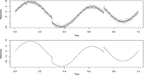
Fig. 2. (Top) Heavisine function and observations and estimates (posterior means) based on the (bottom) recursive and MCMC approaches. The two estimates are almost exact and indistinguishable on the plot. The average square error of the two estimates are 0.0266 and 0.0264, respectively.
which is the mean value of the th power of the explanatory variables .
The reason for this choice of model is that the basis vectors are orthogonal, and for a given segment, the regression parame-ters are independent under the posterior distribution. This helps with the interpretability of the parameter estimates and slightly reduces the computational cost of perfect simulation. The first-and second-order models are obtained by taking the first first-and first two columns of , respectively.
We tested our algorithm on the four test data sets of [16]. These have been previously analyzed by [17] and [1], among others. Each data set consists of 2048 equally spaced observa-tions of an underlying functional relaobserva-tionship (for example, see Figs. 1 and 2). The noise variance was 1.0 throughout, which gives a signal-to-noise ratio of 7 in each case. In our simulation study, we focused primarily on the computational aspects of our approach. The accuracy of inference from a related model to the one we use for these test data sets is given in [1].
We set as in [1]. Initial parameter values were
, , and . We first tried the
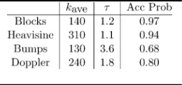
[image:4.594.38.262.611.768.2]TABLE I
RESULTS OFANALYSIS OF THEFOURTESTDATASETS
Section II-C, we used proposals from the posterior distribution conditional on .
In calculating the s for each data set, we truncated the sum in (2) when (3) was less than . By varying this cutoff, we could tell that any inaccuracies introduced were negligible. For each data set, evaluating the recursions to calculate the
s took less than 10 sec on a 900-MHz Pentium PC. Summaries of the computational aspects of the perfect simu-lation and the MCMC algorithms are given in Table I. These in-clude the average number of terms calculated in the sum of (2) ; the autocorrelation time of the MCMC algorithm , and the acceptance probability of the independence sampler. The autocorrelation time was calculated as the maximum estimated time for all the prior parameters.
The average number of terms calculated for the sums in (2) was much less in all cases than the roughly 1000 that would occur if no truncation of the sum was used. The average number of terms depends primarily on the average length of the seg-ments for realizations that have non-negligible posterior proba-bility. For example, the Heavisine function had fewest segments (as few as 5) and, hence, the most terms, whereas, for example, Bumps had many more segments (at least 35) and, thus, fewer terms.
The MCMC algorithm mixed extremely well in all cases. The acceptance probabilities of the independence sampler in part a) of the algorithm were high (close to 1 for Blocks and Heavisine). The autocorrelation times were also low because they were close to 1 for Blocks and Heavisine, which suggests near iid samples from the target posterior distribution.
For each dataset, the estimates based on the recursive ap-proach and those based on the MCMC apap-proach were almost identical. For example, the two estimates for the Blocks and the Heavisine data sets are shown in Figs. 1 and 2. The average mean square errors of the estimates were also almost identical in all cases. As can be seen from these figures, the reconstruction of the Blocks and Heavisine functions are very good.
B. Auto Regressive Processes
Our second example is based on an analyzing data from a piecewise constant AR process. Such models are used for speech data [18]. We considered models of order up to 3. For a segment consisting of observation , the matrix of basis vectors for the third-order model is
..
[image:5.594.101.231.103.164.2]. ... ...
Fig. 3. (Top) Simulated AR process and (bottom) the posterior distribution of the position of the changepoints. The true changepoint positions are denoted by dashed lines.
TABLE II
MAP ESTIMATES OFCHANGEPOINTS ANDMODELORDER
Fig. 4. (Top) Speech data with conditional MAP estimates of the changepoints given by vertical dashed lines and (bottom) posterior distribution of the changepoint positions.
The matrices for the first- and second-order models consist of the first and first two columns of , respectively.
We simulated 2000 data points from a model with nine break-points. The data is shown in Fig. 3. We only used the recursive approach to analyze this data, as the MCMC approach had pro-duced a negligible difference for the polynomial regression ex-amples.
[image:5.594.100.232.712.766.2]TABLE III
CHANGEPOINTPOSITIONS FORDIFFERENTMETHODS
Fig. 5. Changepoint positions of the conditional MAP estimate (solid lines) and those estimated by Punskayaet al.(dashed lines).
The MAP estimate of the changepoint positions and model orders consists of only eight changepoints, whereas the MAP estimate of the number of changepoints is 9 (posterior proba-bility 0.48). The MAP estimates given in Table II are conditional on there being nine changepoints. For the unconditional MAP estimate, the seventh changepoint is missed, but otherwise, the estimates of the changepoint positions and model orders are un-changed. The MAP estimate incorrectly infers the model order for segments 7 and 8. In each case, the MAP estimate is one less than the true model order, and the AR coefficients that are incorrectly estimated as 0 are both small (0.1 and 0.2).
C. Speech Segmentation
We also used our method to analyze a real speech signal [19], which has also previously been analyzed in the literature [1], [18], [19]. We analyzed the data under a piecewise AR model that allowed the AR orders of between 1 and 6 for each segment. We implemented the recursive approach, where an initial run of the exact simulation algorithm is used to construct suitable prior parameters.
The signal, MAP estimates of the changepoints, and posterior distribution of the changepoints are given in Fig. 4. A compar-ison of our estimates of the changepoint positions to previous esimates are shown in Table III, where we give our MAP esti-mates, both conditional and unconditional, on the MAP estimate for the number of changepoints.
Our MAP estimates are similar to those of Punskayaet al. [1], except for the inclusion by the conditional MAP estimate of an extra changepoint near the beginning of the signal and the inclusion by both MAP estimates of an extra changepoint near the end of the signal. Fig. 5 shows these two regions and the estimated changepoints from the different methods.
IV. CONCLUSION
We have presented a novel algorithm for performing exact Bayesian inference for regression models, where the underlying function relationship consists of independent linear regressions on disjoint segments. The algorithm is both scalable and easy to implement. It avoids the problems of diagnosing convergence that are common with MCMC methods.
We have focused on models suggested by [1], but the algo-rithm can be applied more generally. The main requirement is that of independence between the parameters associated with each segment.
The regression problem we have addressed involves model uncertainty. In practice, the accuracy of Bayesian inference for such model-choice problems depends on the choice of prior. We considered two approaches to choosing these priors, both based on letting the data inform the choice of prior parameters. In our examples, we found that the simpler of the two (the recursive ap-proach) performs as well as the approach based on introducing hyperparameters, and we would suggest such an approach in practice.
We have also demonstrated how MAP estimates of the changepoints can be obtained. There are two ways of defining the MAP estimate, depending on whether or not the MAP estimate of the number of changepoints is first calculated, and then, the changepoints are inferred, conditional on this number of changepoints. In some cases, these different approaches can give different estimates for the number and position of the changepoints: For example, when there is a likely changepoint in some period of time but there is a lot of uncertainty over when this changepoint occured, conditioning on the MAP number of changepoints will pick up a changepoint during this period of time, but it may be omitted otherwise (see Section III-B). Note that for the related problem of inferring changepoints in continuous time, it would clearly be correct to conditon on the number of changepoints, as it is inappropriate to compare joint densities of positions of changepoints that are of different dimension.
ACKNOWLEDGMENT
The author would like to thank E. Punskaya for providing the speech data.
REFERENCES
[1] E. Punskaya, C. Andrieu, A. Doucet, and W. J. Fitzgerald, “Bayesian curve fitting using MCMC with applications to signal segmentation,”
[2] P. Green, “Reversible jump Markov chain Monte Carlo computation and Bayesian model determination,”Biometrika, vol. 82, pp. 711–732, 1995. [3] P. Fearnhead. (2004) Exact and Efficient Inference for Multiple Changepoint Problems. [Online]. Available: http://www.maths.lancs.ac.uk/~fearnhea/
[4] L. R. Rabiner and B. H. Juang, “An introduction to hidden Markov models,”IEEE Acoust., Speech, Signal Process. Mag., vol. ASSP-34, no. 1, pp. 4–15, Jan. 1986.
[5] D. Barry and J. A. Hartigan, “Product partition models for change point problems,”Ann. Statist., vol. 20, pp. 260–279, 1992.
[6] , “A Bayesian analysis for change point problems,”J. Amer. Statist. Soc., vol. 88, pp. 309–319, 1993.
[7] J. G. Propp and D. B. Wilson, “Exact sampling with coupled Markov chains and applications to statistical mechanics,” inRandom Structures Algorithms, 1996, vol. 9, pp. 223–252.
[8] C. C. Holmes and D. G. T. Denison, “Perfect sampling for the wavelet reconstruction of signals,”IEEE Trans. Signal Process., vol. 50, no. 2, pp. 337–344, Feb. 2002.
[9] P. D. O’Neill and G. O. Roberts, “Bayesian inference for partially ob-served stochastic epidemics,”J. R. Statist. Soc., ser. A, vol. 162, pp. 121–129, 1999.
[10] P. Fearnhead and L. Meligkotsidou, “Exact filtering for partially-ob-served continuous-time Markov models,”J. R. Statist. Soc., ser. B, vol. 66, pp. 771–789, 2004.
[11] P. J. Green, “Trans-dimensional Markov chain Monte Carlo,” in
Highly Structured Stochastic Systems, P. J. Green, N. L. Hjort, and S. Richardson, Eds. Oxford, U.K.: Oxford Univ. Press, 2003.
[12] J. M. Bernardo and A. F. M. Smith,Bayesian Theory. Chichester, U.K.: Wiley, 1994.
[13] S. Richardson and P. J. Green, “On Bayesian analysis of mixtures with an unknown number of components,”J. R. Statist. Soc., ser. B, vol. 59, pp. 731–792, 1997.
[14] B. P. Carlin, A. E. Gelfand, and A. F. M. Smith, “Hierarchical Bayesian analysis of changepoint problems,”Appl. Statist., vol. 41, pp. 389–405, 1992.
[15] A. J. Viterbi, “Error bounds for convolutional codes and an asymptoti-cally optimum decoding algorithm,”IEEE Trans. Inf. Theory, vol. IT-13, no. 2, pp. 260–269, Apr. 1967.
[16] D. L. Donoho and I. M. Johnstone, “Ideal spatial adaptation by wavelet shrinkage,”Biometrika, vol. 81, pp. 425–455, 1994.
[17] D. G. T. Denison, B. K. Mallick, and A. F. M. Smith, “Automatic Bayesian curve fitting,”J. R. Statist. Soc., ser. B, vol. 60, pp. 333–350, 1998.
[18] F. Gustafsson,Adaptive Filtering and Change Detection. New York: Wiley, 2000.
[19] M. Basseville and I. V. Nikiforov,Detection of Abrupt Changes: Theory and Applications. Englewood Cliffs, NJ: Prentice-Hall, 1993. [20] M. Basseville and A. Benveniste, “Design and comparative study of
some sequential jump detection algorithms for digital signals,”IEEE Trans. Acoust., Speech, Signal Process., vol. ASSP-31, no. 2, pp. 521–535, Apr. 1983.
[21] U. Appel and A. V. Brandt, “Adaptive sequential segmentation of piece-wise stationary time series,”Inf. Sci., vol. 29, pp. 27–56, 1983.
Paul Fearnheadreceived the B.A. and D.Phil. de-grees in mathematics from the University of Oxford, Oxford, U.K.