Improved proposal distribution with gradient measures for tracking

IMPROVED PROPOSAL DISTRIBUTION

WITH GRADIENT MEASURES FOR TRACKING

Paul Brasnett, Lyudmila Mihaylova

_{, David Bull}

_{and Nishan Canagarajah}

Dept. of Electrical and Electronic Engineering

University of Bristol

[email protected], [email protected]

ABSTRACT

Particle filters have become a useful tool for the task of object tracking due to their applicability to a wide range of situations. To be able to obtain an accurate estimate from a particle filter a large number of particles is usually necessary. A crucial step in the de-sign of a particle filter is the choice of the proposal distribution. A common choice for the proposal distribution is to use the transition distribution which models the dynamics of the system but takes no account of the current measurements. We present a particle fil-ter for tracking rigid objects in video sequences that makes use of image gradients in the current frame to improve the proposal distri-bution. The gradient information is efficiently incorporated in the filter to minimise the computational cost. Results from synthetic and natural sequences show that the gradient information improves the accuracy and reduces the number of particles required.

1. INTRODUCTION

Tracking objects in video is an important task due to its ap-plications in diverse areas such as augmented reality, medi-cal applications and surveillance. The general aim of track-ing is to keep track of the pose and location of one or more objects through a sequence of frames.

Particle filtering [1, 2, 3, 4] is a powerful approach for tracking because it makes no assumptions of Gaussian noises and it is able to cope with highly non-linear models de-scribing the image features and system dynamics. Chal-lenges arise when accurate state representations are required in (near) real-time. To obtain results that are accurate a very good model for the proposal distribution is needed. Often the transition distribution is used to model the proposal dis-tribution, this choice does not usually model the proposal distribution accurately so a large number of particles are required. As one would expect increasing the number of particles increases the complexity of the algorithm. This is particularly true for tracking in video sequences because the cost of evaluating the likelihood tends to be high.

∗_{This work has been conducted with support from the UK MOD Data}

and Information Fusion Defence Technology Centre under project DIF DTC 2.2.

There are a number of variants of the particle filter that attempt to address the problem of the proposal distribution. Some of them rely on additional strategies for the proposal distribution such as Monte Carlo Markov chains or the use of gradient information in order to move particles toward more likely regions. The idea of using gradient informa-tion in the proposal distribuinforma-tion has previously been applied to the area of wireless communications [5]. An additional MOVEstep is introduced before the sampling step. The gra-dient information to guide the move to regions of higher likelihood is calculated from the likelihood model.

In [6] the generation of particles is controlled by a mo-mentumterm. Particles with a momentum below a thresh-old are propagated through a deterministic, gradient-descent search the remaining particles are propagated by sampling from the transition density function. An alternative method that moves particles toward regions of higher likelihood is the Kernel Particle Filter [7]. In this approach the mean shift tracker [8] is embedded in a particle filter. Following resam-pling the mean shift iteratively estimates the local likelihood density gradient and moves the particles toward stationary points, which include the modes. The result is that parti-cles are focused around stationary points in the likelihood density.

The aim of the work here is in a similar vein to the works mentioned above, in that gradient information is used to shift the particles. In the present paper an error func-tion is defined and optimised in an efficient gradient-descent method based on the image gradient information available in the frame. In [5] a Levenburg-Marquardt optimisation approach is used whilst here a Newton-Raphson approach to gradient descent allows the development of an efficient implementation. This approach works for a range of linear and non-linear motions, including common motions such as the translation and affine models. The benefit of embedding this in a particle filter framework is the ability to maintain multiple hypothesis, something not possible in a purely de-terministic framework.

model are included in Section 3. A general description of the gradient descent is given in Section 4, from this an ef-ficient gradient measurement for video sequences is devel-oped. The gradient information is incorporated into the par-ticle filtering framework along with implementation details in Section 5. Results are presented in Section 6 and conclu-sions are given in Section 7.

2. PARTICLE FILTERING

Given a system transition functionft:Rn×Rm→Rn

xt+1=ft(xt,wt), (1)

the system state vectorxt∈Rnis estimated at timetwhere

wt∈Rmis a zero mean, white noise sequence independent of past and current states with a known probability density function (PDF).

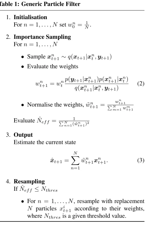
Table 1: Generic Particle Filter

1. Initialisation

Forn= 1, . . . , N setwn

0 =N1. 2. Importance Sampling

Forn= 1, . . . , N

• Samplexn_t+1∼q(xt+1|xnt,yt+1)

• Evaluate the weights

wnt+1=wnt

p(yt+1|xnt+1)p(xnt+1|xnt)

q(xn

t+1|xnt,yt+1)

(2)

• Normalise the weights,w˜n t+1=

wn t+1

PN m=1w

m t+1

EvaluateNˆef f =PN 1 n=1( ˜w

n t+1)2 3. Output

Estimate the current state

ˆ

xt+1=

N

X

n=1 ˜

wnt+1xnt+1. (3)

4. Resampling

IfNˆef f ≤Nthres

• Forn = 1, . . . , N, resample with replacement

N particles xit+1 according to their weights,

whereNthresis a given threshold value.

Measurementsyt ∈ Rp are related to the state vector via the observation equation

yt=ht(xt,vt), (4)

where ht : Rn ×Rr → Rp is the measurement func-tion andvt ∈Rris a different zero mean, white noise se-quence with known PDF, independent of past and present states of the system noise. The Bayesian interpretation of the tracking problem is to recursively calculate a degree of belief in the statextat timet given the measurements

y1:t = {y1, . . . ,yt}. This is represented by the posterior PDFp(xt|y1:t).

The posterior PDFp(xt|y1:t)of the statextis approxi-mated by the particle filter given a measurementy1:tand a set of particlesxn

t each with a corresponding weightwnt

p(xt|y1:t)≈ N

X

n=1

wtnδ(xt−xnt), (5)

where δ(.) is the Kronecker delta function. Each one of the particles xn_t+1 is drawn from the proposal distribution

q(xnt+1|xn0:t,y1:t+1)and assigned a weightwnt+1calculated

recursively at each time step by evaluating the transition densityp(xt+1|xt)the likelihoodp(yt+1|xt+1)and the ev-idenceq(xnt+1|xnt,yt+1). The generic particle filter is given in Table 1.

Note that the resampling stage of Table 1 is necessary to limit the effects of degeneracy [4, 9], the case when only one particle has significant weight.

In the design of a particle filter it is critical to choose a suitable importance density q(xt+1|xn0:t,y0:t+1). A com-mon choice for the importance densityq(xt+1|xnt,yt+1)is to use the transition density

q(xt+1|xnt,yt+1) =p(xt+1|xnt). (6)

This choice only takes into account the system dynam-ics, no account is taken of the measurements. The transition prior is chosen because it leads to a straightforward imple-mentation.

3. LIKELIHOOD MODEL

Weighted colour histogram cues extracted from the frame are used as the result of the measurement function. The weighted histogramHi,xfor biniand statexis given by

Hi,x=CH

X

r_∈Sx

kN

Ã_° ° ° ° ¯

r−r

a ° ° ° °

2!

δi(br), i= 1. . . B,

(7) wherer¯= (¯x,y)¯ is the location of the center pixel,CHis a normalisation constant such thatPB

i=1Hi,x= 1,ais the

size of the kernel,br ∈ {1, . . . , B}denotes the histogram

bins,δi(.)is the Kronecker delta function atiandSxis the

kN, is used to weight pixels in the center of the region more highly than pixels at the edge of the region

kN(r) = (2π)−1/2e− 1

2r. (8)

The Bhattacharyya coefficientρdetermines the distance between two histograms

ρ(Href,Htar) =

B

X

i=1 p

Hi,refHi,tar. (9)

where two normalised histogramsHˆtar andHˆref represent atarget regiondefined in the current frame and areference regionin the frame att0. The Bhattacharyya distance [8]

d(Htar,Href) =

p

1−ρ(Htar,Href), (10)

is a measure of the similarity between these two distribu-tions. The larger the measure ρ(Href,Htar) is, the more similar the distributions are. Conversely, for the distance

d, the smaller the value the more similar the distributions (histograms) are. For two identical normalised histograms we obtaind= 0(ρ= 1) indicating a perfect match.

Based on this distance thelikelihood functionover red, green, blue (R,G,B) colour space can be defined by [10]

p(yt|xnt)∝exp



− X

c∈{R,G,B}

d2(Htarc ,Hrefc ) 2σ2

c



, (11)

for then-th particlexnt. The standard deviationσspecifies the Gaussian noise in the measurements. Note that small Bhattacharyya distances correspond to large weights in the particle filter.

4. GRADIENT INFORMATION

The aim of the gradient descent is to minimise an objective function,O, with respect to the state vectorx,

ˆ

x=arg minxO(x). (12)

IfIt(xt) = [I(r1, t), . . . , I(rR, t)]′ is the vector ofR pixel intensities from an image regionSxt, corresponding to statextat timet. Furthermore the locationsr = [x, y]′ inSxt are determined by the modelg. It is assumed thatg is differentiable with respect to bothrandx.

The objective function can specifically be defined as the following least squares function [11]

O(x) =X

i∈I

(It(xt)−It0(x0))

2_{, (13)}

where x0 is the initial state at time t0. Alternatively the

objective function can be expressed as

O(xt) =kIt(xt)−It0(x0)k

2

. (14)

Reposing the problem in terms of iteratively determin-ing the offsetδxsuch thatxˆt=xt+δxthen (14) becomes

O(δx) =kIt(xt+δx)−It0(x0)k

2

. (15)

If we assume thatδxis small then we can apply contin-uous optimisation procedures to a linearised version of the problem. The problem can be linearised by performing a Taylor series expansion ofIt(xt+δx)aboutxt

It(xt+δx)≈It(xt) +δxMt(xt) +H.O.T., (16)

where H.O.T. refers to higher order terms of the Taylor se-ries expansion andMtis the Jacobian matrix ofItwith re-spect toxt. Making the substitution of (16) into (15) gives

O(δx)≈ kIt(xt) +δxMt(xt)−It0(x0)k

2

. (17)

Solving for _∂∂O_(δx₎= 0and rearranging gives

δx=−(Mt′Mt)−1Mt′[It(xt)−It0(x0)], (18)

and from thisxˆtcan be defined as

ˆ

xt=xt−(Mt′Mt)−1Mt′et, (19)

where

et=It(xt)−It0(x0). (20)

4.1. Efficient Algorithm

Evaluating (19) requires the estimation of the gradient of each target region in every frame. To allow efficient on-line implementation it can be shown that Mt can be de-composed into a time-varying component Σ_t and a con-stantM0, which can be determinedoff-line. The efficiency

comes from removing the need to recalculate the Jacobian

Mtat every iteration. The decomposition ofMtis

Mt(xt) =



   

∇rI(r1, t0)′Γ(r1)

∇rI(r2, t0)′Γ(r2)

.. .

∇rI(r_R, t0)′Γ(r_R)



   

Σ_{t(x) =M0}Σ_t(x),

(21) where ∇rI(r_ℓ, t0)′, ℓ = 1, . . . , R denotes the gradient,

with respect to the components ofr, of pixelrℓat timet0, Σ_t(xt)is dependent upon the motion model used andΓ_(r) depends on both the motion modelgused and the pixel loca-tionr= [x, y]′_{. Examples ofgare given for the translation}

model (Section 4.2) and the affine model (Section 4.3). IfΣ_t is invertible then the state can be moved toward the minimum of the error vectoretby

ˆ

xt=xt−(Σt−1)′Λet (22)

whereΛ_{= (M}′

0M0)−1M0and is computed during an

4.2. Translation Motion Model

The motion model described here and in section 4.3 defines how the pixel locations are related to the state. This first model is for the case when the object performs a translation motion

f(r,xt) =r+xt, xt= [ut, vt]′ (23)

and for this modelM0= [Ix(t0)|Iy(t0)]andΣis the2×2 identity matrix. Remembering thatΛ _{= (M0}T_M0)−1_M0 the updated state,xˆt, at timetis given by

ˆ

xt=xt−Λet. (24)

4.3. Affine Motion Model

If the object to be tracked is a planar object a more suit-able model to capture the transformation is given by the six component affine transform. The motion model and current state of the objectxtat timetcan be described by

f(r,xt) =

· a c b d ¸

r+ ·

u v ¸

=Ar+u. (25)

The state vector is xt = [ut, vt, at, bt, ct, dt]′. Using the affine motion model gives

Γ_{(p) =}

·

1 0 x 0 y 0

0 1 0 x 0 y

¸

, (26)

and

Σ_{t(x) =}





A−1 0 0

0 _A−₁ 0

0 0 _A−1



. (27)

The updated state,xˆt, at timetis given by

ˆ

xt=xt−Σ′tΛet. (28)

It is possible to use other models including some non-linear models. Not all of them are suitable because of the separability property needed to factoriseM.

5. IMPLEMENTATION

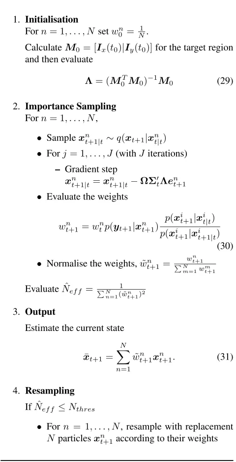
Table 2 presents a particle filter that takes into account the gradient information in the way described in Section 4.

Table 2: Particle Filter with Gradient Step

1. Initialisation

Forn= 1, . . . , N setwn0 =N1.

CalculateM0= [Ix(t0)|Iy(t0)]for the target region and then evaluate

Λ_{= (M0}T_M0)−1_M0 (29)

2. Importance Sampling

Forn= 1, . . . , N,

• Samplexn_t+1|t∼q(xt+1|xnt|t)

• Forj= 1, . . . , J(withJ iterations)

– Gradient step

xn

t+1|t=xnt+1|t−ΩΣ′tΛent+1

• Evaluate the weights

wtn+1=wtnp(yt+1|xnt+1) p(xi

t+1|xit|t)

p(xi

t+1|xit+1|t) (30)

• Normalise the weights,w˜n t+1=

wn t+1

PN m=1w

m t+1

EvaluateNˆef f =PN 1 n=1( ˜w

n t+1)2 3. Output

Estimate the current state

¯

xt+1=

N

X

n=1 ˜

wn_t+1xn_t+1. (31)

4. Resampling

IfNˆef f ≤Nthres

• Forn = 1, . . . , N, resample with replacement

Nparticlesxn

t+1according to their weights

For the purpose of tracking an object in video we ini-tially choose a region which defines the object. The shape of this region is fixeda prioriand in our case it is a rectan-gular box characterised by the state vectorx= (x,x, y,˙ y)˙ ′_,

withxandydenoting the pixel location of the top-left cor-ner of the rectangle, with velocitiesx˙ andy˙. Note that the dimensions of the rectangle are fixed through the sequence.

The transition distributionp(xt+1|xt)used for this work is a constant velocity dynamic model [12]

F = µ˜

F 0 0 _F˜

¶

, F˜ =

µ 1 T 0 1

¶ ,

Q= µ

Qx 0 0 _Qy

¶

, Γ₌

µ1 2T

2 T

¶ ,

with the state vectorx= (x,x, y,˙ y)˙ ′_{, the system noisew=}

(wx′,w′y)′ = (Γ′vx,k,Γ′vy,k)′,vx,k ∽ N(0, σx),vy,k ∽

N(0, σy) being scalar valued zero mean white sequences with standard deviations σx andσy respectively andT is the sampling interval.

The covariance matrices of the noise respectively inx

andycoordinates multiplied by the gain, are

Qx=Γσ2xΓ=

µ1 4T

4 1 2T

3 1

2T 3 _T2

¶ σ2_x.

The covarianceQycan be calculated in a similar way. Suit-able values forσx andσy are ([12], p. 273) in the range

[1

2am, am], withambeing the maximum acceleration.

An implementation issue in combining the constant ve-locity model with the gradient descent is that the gradient descent only updates thexand y coordinates of the state and appropriate account needs to be taken to update the ve-locities. This is done through the use of the following matrix

Ω₌

·

1 _T1 0 0 0 0 1 _T1

¸′

, (33)

whereT is the sampling period and in our implementation

T = 1.

6. RESULTS

The results presented here are from experiments carried out on rigid objects in a natural sequences (Fig. 1) and a syn-thetic sequence (Fig. 2). The object in the synsyn-thetic se-quence is quite textured, in the artificial sese-quence it con-tains more homogeneous regions. The target regions are initialised by providing the coordinates of the target region in the first frame. The statext = (ˆx,y)ˆ represents an esti-mate of the true coordinates(x, y), therefore the root mean squareRM SEis

RM SE=p(xt−xˆt)2+ (yt−yˆt)2. (34) and for a sequence ofFframes it is

RM SEseq=

v u u t1

F

F

X

t=1

(xt−xˆt)2+ (yt−yˆt)2. (35)

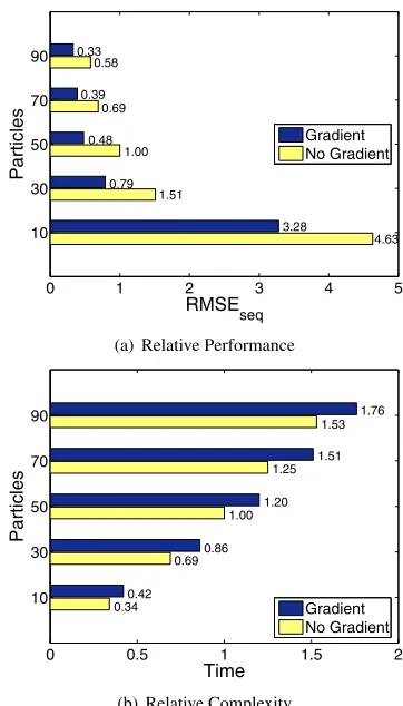
A comparison of the relative performance of the two al-gorithms over the natural sequence is given in Fig. 1. It can be seen that for any number of particles more accurate re-sults are obtained by the particle filter with a gradient step.

0 1 2 3 4 5

90

70

50

30

10

RMSE_seq

Particles

Gradient No Gradient

4.63 3.28

1.51 0.79

1.00 0.48

0.69 0.39

0.58 0.33

(a) Relative Performance

0 0.5 1 1.5 2

90

70

50

30

10

Time

Particles

Gradient No Gradient

1.76 1.53

1.51 1.25

1.20 1.00

0.86 0.69

0.42 0.34

(b) Relative Complexity

Fig. 1. Comparison of the generic particle filter and particle filter with gradient step. All of the results are presented as relative to the generic particle filter with 50 particles (a) Relative RMSE of the state estimated by the algorithm. (b) Relative processing time for the generic particle filter and the particle filter with gradient step. The results are for a sequence of 60 frames and are averaged over 100 runs.

It can also be seen that for comparable complexity the gra-dient particle filter outperforms the generic particle filter. Tracking results of the two algorithms on the natural se-quence are shown in Fig. 3.

Results from a synthetic sequence are shown in Fig. 2. The estimated path from the particle filter is clearly smoother and more accurate when the gradient information is used. This can be clearly seen in Fig. 2a by the jittering in the particle filter path that is not present in when the gradient step is used. TheRM SEcan be clearly seen to be lower when the gradient information is used in Fig. 2b.

7. CONCLUSIONS

distri-95 100 105 110 115 120 125 120

130

140

150

160

170

180

190

200

210

x

y

True PF PF+Gradient

(a) Tracking Results

0 10 20 30 40 50 60

0 0.5 1 1.5 2 2.5 3 3.5 4 4.5

Frames

RMSE

PF PF + Gradient

(b) RMSE

Fig. 2. Comparison of the generic particle filter and particle filter with gradient step applied to an synthetic sequence. (a) A section of the true path of the object compared to the estimates from one run of the particle filter and the particle filter with the gradient step. (b) The RMSE of the particle filter and the particle filter with the gradient step, the results are the mean of 100 run.

bution moves the particles to the high-likelihood regions which results in improved performance. An efficient imple-mentation of the gradient step particle filter is given. Re-sults show that there are two main improvements over a generic particle filter i) a significant increase in the accuracy (lowerRM SE) and ii) since fewer particles are needed to represent the posterior there is a reduction in computational complexity. Future work will extend the method to include changes to the object appearance.

8. REFERENCES

[1] M. Arulampalam, S. Maskell, N. Gordon, and T. Clapp, “A tutorial on particle filters for online nonlinear/non-Gaussian Bayesian tracking,” IEEE Trans. on Signal Proc., vol. 50, no. 2, pp. 174–188, 2002.

[2] J. Liu and R. Chen, “Sequential Monte Carlo methods for dynamic systems,” Journal of the American Statistical As-sociation, vol. 93, no. 443, pp. 1032–1044, 1998.

[3] N. Gordon, D. Salmond, and A. Smith, “A novel approach to nonlinear / non-Gaussian Bayesian state estimation,”IEE

(a) PF (frame 6) (b) PF (frame 54)

(c) PF with Gradient (frame 6) (d) PF with Gradient (frame 54)

Fig. 3. Frames (6 and 54) from a sequence tracking the scoreboard with the two filters. It can be seen that the parti-cle filter with a gradient step results in more accurate track-ing than the generic particle filter.

Proc. on Radar and Signal Processing, vol. 40, pp. 107–113, 1993.

[4] A. Doucet, S. Godsill, and C. Andrieu, “On sequen-tial Monte Carlo sampling methods for Bayesian filtering,”

Statistics and Computing, vol. 10, no. 3, pp. 197–208, 2000.

[5] S. Haykin, K. Huber, and Z. Chen, “Bayesian sequential state estimation for MIMO wireless communications,” Pro-ceedings of the IEEE, vol. 92, no. 3, pp. 439–454, March 2004.

[6] J. Sullivan and J. Rittscher, “Guiding random particles by deterministic search,” inIEEE Int. Conf. on Computer Vi-sion, July 2001, vol. 1, pp. 323–330.

[7] C. Chang and R. Ansari, “Kernel particle filter for visual tracking,” IEEE Signal Processing Letters, vol. 12, no. 3, pp. 242–245, March 2005.

[8] D. Comaneciu, V. Ramesh, and P. Meer, “Kernel-based ob-ject tracking,”IEEE Trans. on Pattern Analysis and Machine Intelligence, vol. 25, no. 5, pp. 564–577, 2003.

[9] A. Kong, J. Liu, and W. Wong, “Sequential imputations and Bayesian missing data problems,” Journal of the American Statistical Association, vol. 89, pp. 278–288, 1994.

[10] P. P´erez, J. Vermaak, and A. Blake, “Data fusion for tracking with particles,” Proceedings of the IEEE, vol. 92, no. 3, pp. 495–513, March 2004.

[11] G. D. Hager and P. N. Belhumeur, “Efficient region track-ing with parametric models of geometry and illumination,”

IEEE Trans. on PAMI, vol. 20, no. 10, pp. 1025–1039, 1998.