Time dependent analysis of virtual waiting time behaviour in discrete time queues

Lancaster University Management School

Working Paper

2005/068

Time-dependent analysis of virtual waiting time behaviour

in discrete time queues

A Wall and D Worthington

The Department of Management Science

Lancaster University Management School

Lancaster LA1 4YX

UK

© A Wall and D Worthington

All rights reserved. Short sections of text, not to exceed two paragraphs, may be quoted without explicit permission,

provided that full acknowledgement is given.

Time-Dependent Analysis of Virtual Waiting Time Behaviour in Discrete

Time Queues

A. D. Wall,1 D. J. Worthington2

1

Faculty of Technology & Environment, Liverpool John Moores University, Byrom Street, Liverpool, L3 3AF, UK. Email: [email protected]

2

Department of Management Science, The Management School, Lancaster University, Lancaster, LA1 4YX, UK. Email:[email protected]

Abstract: Discrete time queueing models have been shown previously to be of practical use for modelling the approximate time-dependent behaviour of queue length in systems of the form M(t)/G/c. In this paper we extend these models to include the time-dependent behaviour of virtual waiting time.

Key components of this research are the derivation of exact (algorithmic) expressions for virtual waiting time behaviour. Statistical approximations for the distributional form of virtual waiting times are then developed and tested. These approximations reduce the computational effort involved in the evaluation of the exact

expressions by a factor of over 1000 whilst still maintaining very high accuracy levels.

The models have been implemented for use on a PC and are shown to be capable of modelling the time-dependent virtual waiting time behaviour of realistic queueing systems in just a few seconds.

Results from the models are compared with results obtained by the Simple Stationary Approximation, the Pointwise Stationary Approximation and Modified Offered Load approximations. They clarify further some of the strengths and weaknesses of these approaches and demonstrate the potential of the Discrete Time Modelling approach.

Keywords: Queueing, Discrete Time Models, Time Dependent Queues, Customer Waiting Time 1. Introduction

Queueing theory and queueing models have provided insights into many industrial and service situations. Most of this analysis assumes constant parameter values and that steady-state results are appropriate. However there are many real queueing situations where parameters vary with time, or where, although parameters are constant, the effects of starting conditions are important.

Analytic models have been developed to examine basic queueing systems that are not in equilibrium. Examples of such models for M(t)/M(t)/∞, M(t)/M(t)/1/1 and M(t)/M(t)/1/∞ are discussed by Gross and Harris [12] and Zhang [25]. Sharma [20] has produced a solution for the transient behaviour of M/M/1 queues. However even for these relatively simple systems, the models are quite complex. If the lack-of-memory property is relaxed or the number of servers increased, the models become more complicated, Choudhury et al. [3].

In practice the choice for queue modelling of time-dependent systems is often between steady-state based approximations and Monte Carlo simulation. In Monte Carlo simulation, the entire distribution of state

no assumptions about the types of arrival and service distributions. However, a lot of computational effort is required to get results.

On the other hand steady-state results are typically much easier to obtain and can provide results that, whilst often biased, are nevertheless sufficiently accurate for decision-making. One popular method of using steady-state results is as a Simple Stationary Approximation (SSA), in which a simple average arrival rate is used to derive steady-state results as an approximation for the overall behaviour of the system. This approach can be valuable if used carefully, but it can also lead to serious errors. For example Eick, Massey & Whitt [6] show that using the steady-state result for the M/G/∞ queue to approximate the M(t)/G/∞ queue with sinusoidal arrival rates provided the correct overall mean number in the system. However it obviously misses the time dependent and hence distributional form of number in the system. For systems with finite numbers of servers, particularly when the servers are often all busy, the non-linear relationship between congestion and traffic intensity implies that the overall congestion in the system for a M(t)/G/c model will generally be underestimated by a M/G/c approximation. For example Green, Kolesar & Svoronos [10] found that using the steady-state M/M/c model to approximate an M(t)/M/c system where actual arrival rate was sinusoidal and varied by only 10% about its average resulted in significant underestimations.

Green, Kolesar & Svoronos [11] and Green & Kolesar [9], in two linked papers, go on to describe and evaluate a Pointwise Stationary Approximation (PSA). Basing their arguments on extensive empirical results for M(t)/M/c systems, they concluded that when it existed the PSA would provide an upper bound on a number of performance measures, and that for a broad range of systems it could be expected to provide reasonably accurate estimates of performance measures. They also identified circumstances in which it was expected to provide poor results.

One clearly identified weakness of a PSA is that it implies that peaks of congestion coincide with peaks in arrival rates, whereas in many real systems the congestion peak lags behind the arrival rate peak. Various methods stemming from the modified offered load (MOL) work of Jennings, Mandelbaum, Massey & Whitt [13], attempt to correct for this by using some weighted average of arrival rates during some period close to time t as an ‘effective’ arrival rate for the PSA model at time t. See for example Green and Kolesar [8] and Green, Kolesar & Soares [10].

An alternative approach for time-dependent queues is to approximate the behaviour using discrete time queueing models. The study of discrete time queues can be traced back to Meisling [14], who studied a single-server system with binomial arrival distribution. Single-single-server systems with random arrivals were analysed algebraically by Dafermos and Neuts [5] and in terms of numerical analysis by Neuts [17]. The Discrete Time Modelling (DTM) approach in which discrete time models are used to approximate the behaviour of continuous time queues was investigated by Omosigho & Worthington [18, 19] for single-sever queues. Brahimi &

Whitt [22, 23] has also found moment matching between continuous service time distributions to be a valuable approach for steady-state behaviour of queueing networks.

From the viewpoint of the customer, waiting time and queueing time are generally more important than queue length. Indeed, for many practical queueing systems service standards are set or monitored in terms of customers’ queueing time, often with a target of X% of customers needing to start service within T minutes of arrival. The main purpose of this paper is therefore to develop models for the time-dependent behaviour of waiting time for discrete time queues.

This paper restricts its analysis to queues with a simple time-dependent Markovian arrival rate, a general service distribution and FIFO (First In/First Out) queue discipline. Whilst these models have wide general application in practice, more complex discrete time models also warrant attention. For example, researchers have studied steady-state waiting time of discrete batch arrival distributions with different queue disciplines, Frigui et al. [7], and a discrete time priority queue, Alfa [1].

The remainder of this paper is organised as follows. Assumptions, notation and definitions are introduced in section 2. Waiting time is to be studied in terms of virtual waiting time, which is introduced in section 3. The development of the virtual waiting time model is in section 4. A crucial element of the set of equations that are obtained are expressions for the distribution of waiting time conditional on the system state. Unfortunately whilst these expressions, and hence the set of equations, are in principle straightforward to solve, in practice they become a prohibitively large computational task for anything but very small parameter values. Section 5 therefore proposes an easily computed statistical approximation for the conditional waiting time distributions, which are shown in section 6 to provide highly accurate results for a tiny fraction of the computational cost. Section 7 is used to demonstrate some of the potential of the DTM approach by using it to calculate the ‘exact’ time-dependent behaviour of virtual waiting time for a discrete time queueing system. This example is also used to shed further light on the strengths and weaknesses of the SSA, PSA and MOL approximation as methods to analyse the time-dependent behaviour of queueing systems. Finally the main conclusions from the paper are summarised in section 8.

2. Assumptions and Definitions

2.1 Assumptions

The discrete time multi-server queue with time-dependent arrival rate and discrete service distribution has the following assumptions:

(ii) The arrival process has a fairly general distribution; the only requirement on the arrival process is that the probability distribution of the number of arrivals in a slot can be calculated and is independent of arrivals in other slots. The arrivals are assumed to enter the system at the end of the slot in which they arrive. This assumption allows for quite a wide class of arrival processes; e.g. homogeneous and inhomogeneous Poisson processes, scheduled arrivals.

(iii) The service times of successive customers are independent and identically distributed random variables measured in terms of the basic unit defined above, with maximum value m. Si = probability (service time takes i discrete time units), for i = 1, 2, ...m. Because arrivals only enter the system at epochs, all services also start and finish at epochs.

(iv) The arrival and service processes are independent. (v) The service system consists of c channels.

(vi) At most one customer can be served in one channel at one time.

(vii) If a customer arrives to find all servers busy he joins a FCFS (First come, first served) queue.

2.2 State-space definition

With these assumptions, discrete time multi-server queues can be formulated as time-inhomogeneous Markov chains, as shown by Brahimi & Worthington [2], using a state system thatconsists of all possible vectors of the form

(

n

:

x x

₁

,

₂

,..

x

_m

)

c

subject to

x

i

n

i m

=

=

∑

1

min( , )

where n = 0, 1, 2, ... records the number in the system, and the are non-negative integers recording the number of services in process that have exactly i units of time remaining.

x

_i

For ease of notation we then simply list the states associated with any number (n) in the system so that they can be numbered j=1, 2, ...The number of states associated with each n is:

(

)!

!(

)!

(

)

(

)!

!(

)!

(

)

n

m

n m

n

c

c

m

c m

n

c

+ −

−

<

+ −

−

≥

⎧

⎨

⎪⎪

⎩

⎪

⎪

1

1

1

1

Hence the state-space {

(

,

}can now be abbreviated to {(n,j)}, where for any given n value, each j value corresponds to a unique combination of service times remaining. The stochastic behaviour of the system over time can then be described by {p_n,j,t}, where

,..

n

:

x x

_{1 2}

x

_m

)

Methods to find {pn,j,t} are already known, see for example Brahimi & Worthington[2].

2.3 Other Definitions

Two probability functions based on the service time distribution are required later and are introduced here for convenience.

Ω(T): the probability that a service time lasts more than T. Thus:

Ω

( )

T

S

T

T

m

i i T m

=

−

≥

⎧

⎨

⎪

⎩⎪

= +

∑

for = , ,...,

for

0 1

1

0

1

m

Ψ(N)

(T): the probability that N service times take a total of exactly T time units. As this is the Nth convolution of the service time distribution, Ψ(N)(T) can be calculated as:

Ψ

( )

( )

!

!

N i N i i m

T

N

S

N

i

=

=

∏

∑

1

for T = N, N+1,…..,Nm

where the summation is taken over all combinations of non-negative integers {N_i} for which

.

and

,

1 1

∑

∑

= =

=

=

m i i m i

i

N

i

N

T

N

3. Virtual Waiting Time Distribution

Virtual waiting time at time t is defined to be the time that an imaginary customer would have to wait before service if they arrived in a queueing system at instant t. Gross and Harris [12, section 2.3] give a derivation of the steady-state virtual waiting time distribution for an M/M/c model. However the virtual waiting time concept does not just apply to steady-state systems as shown by Minh [16] for M(t)/G/1. The virtual waiting time distribution was first formulated for discrete time queues by Neuts [17] for the single server case.

Combining these ideas, the probability distribution of virtual waiting time at time t, w_t( ), in a c server discrete time system with system states as defined earlier can be expressed as:

(4b)

.

at time

)

,

(

state

in

system

found

arrival

/

at time

occurs

completion

service

th

)

1

(

Pr

)

(

0

>

for

and

(4a)

)

0

(

)! 1 ( ! )! 1 ( 1 , , 1 0 )! 1 ( ! )! 1 ( 1 , ,

∑ ∑

∑ ∑

≥ − − + = − = − − + =

⎭

⎬

⎫

⎩

⎨

⎧

−

+

=

=

c n m c m c j t j n q q t q c n m n m n j t j n t

p

t

j

n

T

c

n

T

w

T

p

w

⎭

⎬

⎫

⎩

⎨

⎧

+

=

)

(

state

in

system

found

arrival

/

time

in

s

completion

service

)

1

(

exactly

Pr

)

(

.

n,j

T

n-c

T

WC

_{nj q} q

(5)

so that (4b) simplifies to:

w T

_{t q}

p

_{n j t}

WC

_{n j}

T

_q

T

j n c

q c m

c m

(

)

_{, , ,}

(

)

( ) !

!( )

=

= ≥

+ − −

∑

∑

1

1 1

0

for

>

(6)

Note that WC_n,j(T_q) is conditional only on the state (n,j) and is independent of t. Hence conversion of the queue length distributions into time dependent virtual waiting time behaviour reduces to the non-trivial problem of deriving methods for obtaining the conditional waiting time distribution WC_n,j(T_q) for all (n,j). This step is developed next in sections 4, 5 and 6.

4.

An Exact Method

4.1 Single Server Formulation and Solution

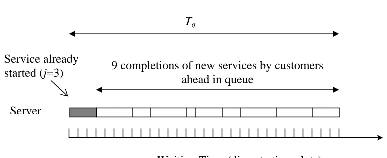
We first consider the single server queue, as previously formulated by Neuts [17]. Our formulation differs a little from that of Neuts in preparation for the multi-server formulation that follows. For the single server system the state (n,j) when n>0 indicates that there are n in the system and that the residual service time of the one customer in service is j. Hence there will be exactly n-c+1 = n completions in time T_q if and only if there are n-1 complete service times in the time remaining after the customer in service has completed its current service, i.e. in time (Tq- j). Using the probability function introduced earlier, this has probability Ψ

(n-1)

(Tq- j).

[image:7.595.69.456.539.697.2]

This formulation is shown diagrammatically in figure 1 for the case of a virtual customer arriving to find the system in state (n,j) = (10,3), i.e. 3 time units left for customer in service and another 9 customers ahead in queue.

Figure 1: Single-server example of virtual waiting time

T

q

Service already

started (

j

=3)

9 completions of new services by customers

ahead in queue

Server

Waiting Time (discrete time slots)

WC

_{n j,}

( )

T

_q

=

Ψ

(n−1)

(

T

_q

−

j

)

4.2 Multi-Server Formulation and Solution

In the multi-server system the problem is more complicated in two main ways. Firstly, there are now c channels contributing to the total number of completed service times. The second consideration is that only one of the c servers needs to complete a service at the time Tq of interest. The other (c-1) servers may complete their

contributing service times at time Tq or before. This second consideration adds greatly to the complexity of the

formulation of the problem. An algorithmic form of solution has been developed and is outlined below. For further details see Wall [21].

For any state (n,j), where n≥c,it is possible to define a unique numbering of the servers (i = 1, 2, .. c) by requiring that they are ordered

s

j,1

≤

s

j,2

≤ ≤

K

s

j c, , where sj,iis the residual service time of the customer

currently with server i. Ties are settled by some predefined order of the servers. The imaginary customer arriving to find the system in state (n,j) is then assumed to go into service with the lowest numberedserver available at time Tq. We can therefore consider each of the c servers individually for i = 1, 2, ...c and define a

probability function:

SC

T n TF

server i

n

T

TF

n j

n j i q i i i q

i

, ,

(

,

,

)

Pr{

, )}

=

completes services by time

and last completion

occurs at

/ arrival found system in state (

(where TFi = 0 if ni = 0)

Note that this probability function specifically recognises the possibility that the time TFi at which server i

completes his nithservice may well be before the time Tq that is of interest.

This formulation is shown diagrammatically in figure 2 for the case of a c=3 server system and a virtual customer arriving to find the system in state (n,j) = (17,jj) where jj implies that the three residual service times are 2, 3 and 3 units respectively (sjj.1 = 2, sjj.2 = sjj.3 = 3). In this example as there are 17-3=14 customers ahead,

the virtual customer will end up in service with server 1, with this combination of services.

Figure 2: Multi-server example of virtual waiting time

T

q

Services

already started

(

s

j.i

)

Server

TF

1

TF

2

TF

3

1 2 3

For the general case for any server i,if s_j,i > Tq, (i.e. the residual service time of server i, given system starts in

state (n,j), is larger than Tq) then trivially:

SC

n j i

T n TF

q i i

n

TF

i i , ,

(

,

,

)

=

=

⎧

⎨

⎩

1 when

= 0 and

0 otherwise

0

Whereas if

s

_{j i,}

≤

T

_q, using the distribution functions introduced in section 2.3:

SC

T n TF

TF

s

T

TF

TF

T

T

s

TF

T

n j i q i i

n

i j i q i i

n

q j i i

i i , , ( ) , ( ) ,

(

,

,

)

(

). (

)

(

)

=

−

−

−

=

⎧

⎨

⎪

⎩⎪

− −

Ψ

Ω

Ψ

1 1

for

for

q q

<

Now considering all c servers together, define

⎟

⎟

⎟

⎠

⎞

⎜

⎜

⎜

⎝

⎛

=

)

,

(

state

in

system

found

ly/arrival

respective

,...,

,

at

s

completion

last

their

with

time

by

services

...

,

,

completed

have

1,2,....,

Servers

Prob

})

,

{

,

(

_{1 2}

2 1 / ,

j

n

TF

TF

TF

T

n

n

n

c

TF

n

T

WC

_{q c}

c i i q j n

Because of the independence of the c service processes when they are all working continuously, we can say that:

∏

=

=

c i i i q i j n i i q j

n

T

n

TF

SC

T

n

TF

WC

1 , , / ,

(

,

{

,

})

(

,

,

)

Finally, we note that

∑

=

* * / ,

,j

(

q

)

n j

(

q

,

{

i

,

i

})

n

T

WC

T

n

TF

WC

(7)

**

where the summation is over all combinations of {ni, TFi} such that

and

{ }

_∑

=

+

−

≥

=

=

c i i i

q

TF

n

k

n

c

T

1 c

1 =

i

,

1

max

q

i

T

TF

=

for more than

k

−

(

n

−

c

−

1

)

servers.

Hence the conditional waiting time distribution

WC

can also be evaluated for multi-server systems. Note that the evaluation of equation (7) requires all feasible combinations of {ni,TFi} to be generated once.

T

n j,

(

q

)

4.3 The Need to Approximate the Conditional Waiting Time Distributions.

Neuts [17] noted that his single server discrete time algorithms needed further approximations particularly with regard to the waiting time distribution in order to make the technique practical on a mainframe computer. Nowadays, the increased computing power of a personal computer means that the methods described above are practical for single server systems. However for multi-server systems the time to compute the conditional waiting time probabilities increases dramatically, and becomes prohibitively long for modest numbers of servers. We therefore developed a practical approximation approach to reduce the computational requirements and hence extend the range of c that can be analysed for any given level of computing power. This approach is described next.

5. Overview of the Approximation Approach

shown in figure 3. As n increases from 6, through 10, 15 and 25 to 40 the shape can be seen to start rather skewed and irregular but becoming more regular and more symmetric. The approximation approach therefore sought to fit a standard distribution to WC_n,j(T_q) for ‘high’ n (i.e. for n>Q, where Q is some ‘high’ value chosen by the analyst) which could then be used to estimate the individual probabilities directly, rather than calculate them from the exact equations given earlier.

Figure 3: Typical Conditional Waiting Time Distributions _WCn,j(_Tq) For One Example j.

3 server system

0 0.2 0.4 0.6 0.8 1 1.2

Waiting time (units of discrete time)

pdf probability

6 10 15

25 40

n : no. of customers in the system

The requirement was therefore for a family of distributions which could represent this type of distributional behaviour and for which the pdf or cdf could be evaluated easily. Discrete distributions would be consistent with the discrete time basis of the models, but the obvious candidates were computationally expensive to evaluate. Hence continuous distributions were considered, and in particular the Gamma distribution, with pdf:

f x

k

x

e

k

x

k

k k k x

( )

(

)

( )

,

,

,

, ....

=

θ

−1 −θ

>

0

θ

>

0

1 2

Γ

for

=

which is well-known to have the observed shape characteristics.

In order to discretize a Gamma distribution the probability of a discrete value Tq was taken to be the probability

of the continuous variable taking values in the range (Tq-0.5, Tq+0.5), i.e.

(8)

WC

_{n j}

T

_q

f x dx

T T

q q

,

. .

(

)

=

( )

− +

∫

0 5 0 5

The selection of an appropriate Gamma distribution was done on the basis of matching its mean,

1

_θ

to a target mean, and matching its variance,

1

₂

k

θ

as closely as possible to a target variance. Once θ and k were

calculated, evaluation of (8) using numerical integration quickly led to a discretized version of the Gamma distribution (referred to as ‘Uncorrected Variance’ later).

Miller and Rice [15] have shown that the mean of a discretized distribution will not always equal the continuous mean,

1

_θ

, but more interestingly that its variance will be larger than the continuous variance,

1

₂

k

θ

. Hence

a system with a slightly larger k than the one chosen by the method outlined above may provide a slightly better match. Our second method of choosing a discretized Gamma distribution (referred to as ‘Corrected Variance’ later) investigates this effect.

In addition two methods of performing the numerical integration were investigated. In the first the area under the curve is approximated by a single trapezoidal shape using:

[

(

0

.

5

)

(

0

.

5

)

]

2

1

)

(

.j q

≈

q

−

+

q

+

n

T

f

T

f

T

WC

In the second, the accuracy of integration is improved by taking an additional point (i.e. midpoint). This takes about twice as long to compute. Assuming the curve through the three points is a parabolic shape (as in Simpson’s First Rule) we therefore use:

[

(

0

.

5

)

4

(

)

(

0

.

5

)

]

6

1

)

(

.j q

≈

q

−

+

q

+

q

+

n

T

f

T

f

T

f

T

WC

Finally, and crucially, reasonably accurate estimates of the mean and variance of the distribution WC_n,j(T_q) are required so that a Gamma distribution can be chosen. A near exact equation for predicting the mean is described in section 5.1. A similar equation for the variance is described in section 5.2.

Overall we observe that this approach to approximating the conditional waiting time distribution for higher values of n turns out to be highly practical for three important reasons:

1) The time spent obtaining the conditional waiting time distribution in the full model is mainly spent running that portion which contains higher values of n. Hence the runtime savings from a scheme that only runs the full model for small n will be very large.

2) In many practical queueing systems (e.g. those with low and medium loads), most of the customer probability is associated with low n. It is therefore more important to model the system as accurately as possible for low n. Any errors due to approximating the high n portion of the system will have a much less significant effect. This was also an observation of Neuts [17] for single server systems.

3) As will be seen later, the mean and variance of conditional waiting times showed strong patterns with increasing n, perhaps associated with Central Limit Theorem behaviour Thus it was possible to deduce very good predictive models for the mean and variance.

In order to obtain estimates of the mean of the conditional waiting time distribution we derive an expression for sum of all the remaining services times to be experienced by the customers in the system when an arbitrary arrival arrives to find state (n,j) where j implies the unique set of residual service times , which for ease of notation in this section are simplified as s

s

_j,1

≤

s

_j,2

≤ ≤

_K

s

_{j c,}

1,…..,sc.

The sum of the remaining service times will be:

∑

∑

−

= =

+

n c

i i c i i

S

s

1 1

Another way of deriving the same total amount of time would be to use the total wait experienced by the arbitrary arrival Tq, and the residual service time on the remaining (c – 1) servers who are still busy when the

arrival goes into service:

∑

−

+

c1

i i

q

R

cT

where Ri is the residual service time on server i.

Therefore:

∑

∑

∑

(9)

− − = =

+

=

+

1 1 1 c i i q c n i i c i

i

S

cT

R

s

Taking the expected values of (9) gives:

(10)

)

(

)

1

(

)

(

)

(

)

(

1

R

E

c

T

cE

S

E

c

n

s

q c i

i

+

−

=

+

−

∑

=

To find an approximation for E(R) we make the assumption that the values of Ri (for i= 1,2, …,c-1) are

independent of each other and of Tq , and hence are equivalent to the limiting forward recurrence times in a

renewal process where the renewal time is our service time. Hence, as shown by Cox [4], the pdf of R is:

)

(

)

(

1

S

E

x

F

_s

−

And:

2

)

(

)

1

(

)

(

2

)

(

)

(

2

S

E

SCV

S

E

S

E

R

E

=

=

+

(11)

12

)

(

)

)

(

2

)

(

1

(

2

)

(

)

(

3

)

(

)

(

2 2

S

E

S

E

S

Var

S

Var

S

E

S

skewness

R

Var

=

+

−

+

(12)

where the expression for Var(R) can be simplified as:

Substituting (11) in (10) and rearranging gives our estimate of E(Tq):

∑

=

+

⎟

⎠

⎞

⎜

⎝

⎛

−

+

+

−

−

=

c

i i

q

s

c

S

E

c

SCV

c

c

n

T

E

1 2

1

1

)

(

)

1

)(

1

(

)

1

2

(

)

(

ˆ

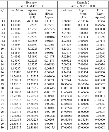
Table 1: Comparison Of Exact And Approximate Means Of Conditional Waiting Time Distributions for a 3 server system, sub-state (j=1) for two example service time distributions tabulated in Table 2

Example 1 m = 4, SCV = 0.333

Example 2 m = 7, SCV = 1.000 n.j Exact Mean Approx

Mean (13)

Error (Exact-Approx)

Exact mean Approx Mean

(13)

Error (Exact-Approx) 3.1 1.00000 -0.11110 1.11110 1.00000 -0.33334 1.33334

4.1 1.00000 0.72223 0.27778 1.00000 0.33334 0.66666

5.1 1.00000 1.55555 -0.55555 1.00000 1.00000 0.00000

6.1 2.38182 2.38890 -0.00709 2.04888 1.66666 0.38222

7.1 3.18177 3.22223 -0.04046 2.32042 2.33334 -0.01292 8.1 4.03674 4.05555 -0.01881 2.92884 3.00000 -0.07116

9.1 4.92694 4.88890 0.03804 3.61526 3.66666 -0.05140

10.1 5.71476 5.72223 -0.00747 4.23080 4.33334 -0.10254

11.1 6.51544 6.55555 -0.04011 4.93976 5.00000 -0.06024

12.1 7.40363 7.38890 0.01473 5.62400 5.66666 -0.04266

13.1 8.23397 8.22223 0.01174 6.30522 6.33334 -0.02812

14.1 9.03712 9.05555 -0.01843 7.00034 7.00000 0.00034

15.1 9.89237 9.88890 0.00347 7.67230 7.66666 0.00564

16.1 10.73186 10.72223 0.00963 8.34134 8.33334 0.00800

17.1 11.54489 11.55555 -0.01066 9.00756 9.00000 0.00756

18.1 12.38911 12.38890 0.00021 9.67064 9.66666 0.00398

[image:14.595.70.442.105.557.2]

19.1 13.23010 13.22223 0.00787 10.33696 10.33334 0.00362 20.1 14.04940 14.05555 -0.00615 11.00130 11.00000 0.00130 21.1 14.88733 14.88890 -0.00157 11.66648 11.66666 -0.00018 22.1 15.72807 15.72223 0.00584 12.33338 12.33334 0.00004 23.1 16.55236 16.55555 -0.00319 12.99940 13.00000 -0.00060 24.1 17.38677 17.38890 -0.00213 13.66606 13.66666 -0.00060 25.1 18.22627 18.22223 0.00404 14.33298 14.33334 -0.00036 26.1 19.05416 19.05555 -0.00140 14.99966 15.00000 -0.00034 27.1 19.88682 19.88890 -0.00208 15.66658 15.66666 -0.00008 28.1 20.72485 20.72223 0.00263 16.33334 16.33334 0.00000 29.1 21.55518 21.55555 -0.00037 17.00000 17.00000 0.00000 30.1 22.38715 22.38890 -0.00175 17.66674 17.66666 0.00008 Table 2: Discrete Service Distributions Used In Tables 1 & 3

Service Time (slot time units)

Example 1 Probability

Example 2 Probability

1 0.47222 0.66667

2 0.00000 0.20000

3 0.08333 0.00000

4 0.44444 0.00000

5 6 7

0.00000 0.00000

0.13333

5.2 Estimating the Variance of the Conditional Waiting Time Distribution

)

var(

)

1

(

)

var(

)

var(

)

(

0

+

n

−

c

S

=

c

2

T

_q

+

c

−

R

and rearranging for var(Tq) gives:

2

)

var(

)

1

(

)

var(

)

(

)

var(

c

R

c

S

c

n

T

_q

=

−

+

−

(14)

Substitution of (12) into (14) then gives our first estimate of var(Tq). Empirical results showed that this equation

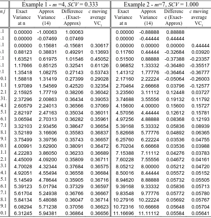
[image:15.595.76.500.313.751.2]

produces reasonably good estimates of the variance for multi-server systems. Table 3 presents results for the same two example test distributions (see table 2) used for demonstration in table 1. The third column in each case shows the error of the approximation formula, which shows that our variance model is not as accurate as the mean model given in section 5.1. It can be seen that while the error initially reduces as n increases, it then tends to become fairly constant as n increases further. The fourth column in each case shows a c-point moving average of the errors which we call VCj. This shows a more consistent error value as n increases.

Table 3: Comparison Of Exact And Approximate Variance Of Conditional Waiting Time Distributions for 3 server system, j=1 for two example service time distributions tabulated in Table 2

Example 1 -

m

=4,

SCV

= 0.333

Example 2 -

m

=7,

SCV

= 1.000

n.j Exact

Variance at n Approx Variance (14) Difference . (Exact-Approx)

c moving average VC₁ Exact Variance at n Approx Variance (14) Differenc e (Exact-Approx)

c moving average

VC₁ 3.1 _{0.00000 -1.00063 1.00063 0.00000 -0.88888 0.88888}

4.1 0.00000 -0.07469 0.07469 0.00000 -0.44444 0.44444

5.1 0.00000 0.15681 -0.15681 0.30617 0.00000 0.00000 0.00000 0.44444

6.1 0.88123 0.38831 0.49291 0.13693 0.11760 0.44444 -0.32684 0.03920

7.1 _{1.63521 0.61975 1.01546 0.45052 0.51500 0.88888 -0.37388 -0.23357} 8.1 1.17666 0.85125 0.32541 0.61126 0.96852 1.33332 -0.36480 -0.35517

9.1 1.35418 1.08275 0.27143 0.53743 1.41312 1.77776 -0.36464 -0.36777

10.1 1.58818 1.31419 0.27399 0.29028 2.17160 2.22224 -0.05064 -0.26003

11.1 _{1.97089 1.54569 0.42520 0.32354 2.70464 2.66668 0.03796 -0.12577} 12.1 2.15925 1.77719 0.38206 0.36042 3.23560 3.11112 0.12448 0.03727

131. 2.37296 2.00863 0.36434 0.39053 3.74688 3.55556 0.19132 0.11792

14.1 2.60579 2.24013 0.36566 0.37069 4.15600 4.00000 0.15600 0.15727

15.1 _{2.82197 2.47163 0.35034 0.36011 4.57056 4.44444 0.12612 0.15781} 16.1 3.06594 2.70313 0.36282 0.35961 4.97256 4.88888 0.08368 0.12193

17.1 3.32103 2.93456 0.38647 0.36654 5.39168 5.33332 0.05836 0.08939

18.1 3.52189 3.16606 0.35583 0.36837 5.82668 5.77776 0.04892 0.06365

19.1 _{3.75499 3.39756 0.35743 0.36657 6.25760 6.22224 0.03536 0.04755} 20.1 4.00991 3.62900 0.38091 0.36472 6.70204 6.66668 0.03536 0.03988

21.1 4.22283 3.86050 0.36233 0.36689 7.15388 7.11112 0.04276 0.03783

22.1 4.45009 4.09200 0.35809 0.36711 7.60228 7.55556 0.04672 0.04161

23.1 _{4.70028 4.32344 0.37684 0.36575 8.05212 8.00000 0.05212 0.04720} 24.1 4.92051 4.55494 0.36558 0.36684 8.50016 8.44444 0.05572 0.05152

25.1 5.14549 4.78644 0.35905 0.36716 8.94620 8.88888 0.05732 0.05505

26.1 5.39123 5.01794 0.37329 0.36597 9.39168 9.33332 0.05836 0.05713

27.1 _{5.61704 5.24938 0.36766 0.36667 9.83548 9.77776 0.05772 0.05780} 28.1 5.84134 5.48088 0.36047 0.36714 10.27916 10.22224 0.05692 0.05767

29.1 6.08294 5.71238 0.37056 0.36623 10.72316 10.66668 0.05648 0.05704

Because equation (14) tends to provide a biased estimate of the required variance, as indicated by the moving average terms, the full method proposed for estimating the variance for largish n is:

j

q

VC

c

R

c

S

c

n

T

=

−

+

₂

−

+

^

₍

₎

_var(

₎

₍

₁

₎

_var(

₎

)

(

var

(15)

where var(R) is estimated using (12) and the correction term VCj is obtained by running the full waiting time algorithm for n up to some limit, say n ≤Q. We then calculate an estimate of the error term _VCj , as in table 3, which is then used in equation (15) for n>Q.

As equation (15) incorporates this empirically derived constant _VCj which depends on the value of Q chosen, the fourth column for each example in table 3 can be interpreted as showing the values of the variance corrections VCj that would result from setting Q at different n. Clearly these stabilise fairly quickly and are typical of other results obtained for other conditional waiting times for a variety of systems, see Wall [21].

6. Evaluation of the Approximation Techniques

6.1 Accuracy

Evidence has been presented in the previous sections to provide some justification for equations (13) and (15) as methods for estimating the mean and variance of conditional waiting times for largish values of n. In this section these formulae are incorporated into the overall approach to approximate the distribution of virtual waiting time.

The results reported here are a summary of more extensive results reported in Wall [21]. In total four different methods of approximation were considered. They were numbered as follows:

Method 1 Trapezium Discretization : Uncorrected Variance Method 2 Trapezium Discretization : Corrected Variance Method 3 Parabolic Discretization : Uncorrected Variance Method 4 Parabolic Discretization : Corrected Variance

For each of these, 18 different test cases were investigated using four different service time distributions, c=2, 3 and 4, ρ ranging from 0.3 to 0.9 and a variety of times (t) at which the virtual waiting time distribution was calculated. The test cases were chosen to produce waiting time distributions that would challenge the waiting time approximation. For example the test cases generally have high congestion levels, which ensures that behaviour for n>Q is important.

Graphical comparisons showed the results were all to a high standard, such that differences between approximate and exact distributions could not be discerned visually. A more rigorous assessment of the numerical accuracy was also performed by comparing both the first four moments of the virtual waiting time distributions and also various percentiles of the distributions (10%, 50%, 70%, 80%, 90%, 95%, 99% and 99.9%). A summary of the results is as follows:

1. For the large majority of the comparisons the accuracy of the approximation techniques was good to 6 or more significant figures.

2. As would be expected the accuracy of all four methods (Methods 1, 2, 3, 4 as above) increases as Q increases.

3. In virtually all cases the approximation is accurate to at least 3 significant figures for all the moments and percentiles for even the lowest level of Q. The only minor exceptions to this were for one test case in its highest moments and highest percentiles, which were only accurate to 2 significant figures at the two lowest levels of Q investigated.

4. The parabolic discretization (methods 3 & 4) was generally superior to trapezium discretization (methods 1 & 2), although not much.

5. In general there was little to choose between the Corrected Variance methods (methods 2 & 4) and the Uncorrected Variance methods (methods 1 & 3).

We conclude that for practical purposes, the trapezium discretization with uncorrected variance is likely to be more than adequate if Q = 2c+10 is used. At this level of accuracy, the higher (third and fourth) moments and higher (99% and 99.9%) percentiles are all within 0.1% of the exact discrete distribution values. The lower moments and percentiles are considerably more accurate than this.

We also observe that there is no evidence that the technique deteriorated as the number of servers increased, and therefore postulate that the technique will continue to achieve high accuracy levels for more than 4 servers. Obviously, increases in approximation accuracy can be achieved by replacing the trapezium method by the parabolic method and by increasing Q. However, this will be at the expense of runtimes as discussed in the next section.

6.2 Runtime Experience

The total runtime associated with the waiting time model first requires the queue length behaviour to be

The benefit in runtime of using the approximate method was considerable. The savings are most dependent on the value of Q, which is the level of n above which the approximation technique is applied. It is clearly beneficial for runtime purposes to keep Q as low as possible, but there is a trade off in decreasing accuracy. In this example, setting Q at 16 reduced the 76.8 minutes to about 6 seconds whilst very good accuracy was maintained, setting Q at 11 took under two seconds and still provided results that would be acceptable for many practical purposes.

The difference in runtimes between the different Corrected and Uncorrected Variance approximation methods was not detectable in this example. The parabolic methods (3 & 4) were slightly slower than the trapezoidal methods (1 & 2) by 0.4 seconds.

These results were obtained on an elderly Pentium 75MHz PC, run as a single task. A modern entry-level machine would be at least 50 times faster than the timings indicated here, but the relative values would persist. However, the runtimes indicated here would be typical on a modern PC if the queueing system contained a higher number of servers and/or higher arrival intensity of the queue

Clearly the time taken to run the exact waiting time model massively inflates the time required to run the original discrete time model for queue length behaviour alone by a factor of about 185. However the methods devised to approximate the waiting time distribution lead to enormous savings. In this example the

approximation methods reduce the inflation factor of providing waiting time results to 1.2 when Q=16 whilst maintaining a very high degree of accuracy.

7. Some Example Results

In this section we demonstrate some of the capabilities of the discrete time modelling (DTM) approach by applying the waiting time model derived in this paper to investigate the extent to which the Simple Stationary Approximation (SSA), the Pointwise Stationary Approximation (PSA) and modified offered load (MOL) based methods can be used to provide useful bounds or approximations on performance measures for queues with nonstationary arrivals. As noted in the introduction, SSA uses steady-state results to approximate time-dependent behaviour, based on an overall average arrival rate. PSA uses steady-state values based on the instantaneous arrival rate. MOL based methods incorporate a time lag by estimating an effective arrival rate at each time point, which is then used in the PSA model.

The examples presented here reinforce the investigations of Green et al. [11] and Green and Kolesar [9] who used mainly empirical results for Markovian queueing systems with sinusoidal arrival rates to indicate conditions under which the SSA and PSA could be used to provide reasonably accurate bounds on behaviour. Our examples also demonstrate the types of situations in which the time-dependent approach presented in this paper would be much better.

same performance measures. Green and Kolesar [9] and Green et al. [10] demonstrated a broad range of systems for which the PSA produces reasonably accurate estimates of performance measures as well as identifying circumstances in which the PSA is not a good approximation.

The example we use here is a queueing system which operates over a cycle that consists of 4 quarters, each of duration of 60 units of time. So for example if 1 unit = 1 minute (case 1), the duration of the cycle is 4 hours which might represent a morning's activity for an office. Alternatively if 1 unit = 6 minutes (case 2), the cycle would be 24 hours long and the activity might be a 24 hour per day service. The arrival rates during each quarter are 0.5, 0.8 , 0.95 and 0.8 per unit time respectively, corresponding to hourly arrival rates of 30, 48, 57 and 48 in case 1 and hourly arrival rates of 5, 8, 9.5 and 8 in case 2. The discrete service time distribution is given in table 4, giving rise to a mean service time of 3 units, i.e. 3 minutes in case 1 and 18 minutes in case 2. There are 3 servers, so the service capacity is 60 per hour in case 1 and 10 per hour in case 2.

Table 4: Discrete Service Time Distribution Used In Cases 1 & 2 Service Time

(units)

Probability

1.0 0.05 2.0 0.3 3.0 0.35 4.0 0.2 5.0 0.1

[image:20.595.90.519.119.335.2]

Figure 4: Waiting Time Statistics Derived From Waiting Time Distribution Over 4 Cycles

0 2 4 6 8 10 12

0

60

120 180 240 300 360 420 480 540 600 660 720 780 840 900 960

Time (Minutes)

Customer W

a

iting Time Mean

50.00% 90.00%

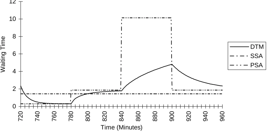
The SSA, PSA and MOL approaches are designed primarily to model systems at cyclic steady-state and so we consider the results for the fourth of the cycles. In figures 5 and 6 predictions of mean virtual waiting time and the 90% percentile of virtual waiting time using the DTM, SSA, PSA and MOL approaches are compared. Note that in this example, whichever MOL based method is used, the effect is only to cause a slight ramping instead of the step changes in congestion levels implied by the PSA model. However the ramps are very steep, are barely discernable from the PSA lines in figures 5 and 6, and are therefore not overlaid on figures 5 and 6.

Figure 5: Comparison Of Mean Waiting Time Derived By The Different Models For 4th Cycle

0 2 4 6 8 10 12

720 740 760 780 800 820 840 860 880 900 920 940 960

Time (Minutes)

Waiting Time

[image:20.595.90.521.534.749.2]

[image:21.595.87.521.141.358.2]

Figure 6: Comparison Of 90% Percentile of Waiting Time Distribution Derived By The Different Models For 4th Cycle

0 5 10 15 20 25

720 740 760 780 800 820 840 860 880 900 920 940 960

Time (Minutes)

Waiting Time

DTM SSA PSA

In both figures the SSA just predicts one fixed level throughout the cycle. For that section of the cycle for which the average arrival rate exceeds the actual arrival rate (i.e. the first quarter only) the SSA exceeds the PSA (& MOL), for the other three quarters the PSA exceeds the SSA. Furthermore the non-linear relationship of measures of congestion to traffic intensity means that the overall mean delay according to the PSA, see table 5, will be greater, in this case considerably greater, than that according to the SSA. Table 5 shows this relationship clearly for overall mean queue length and also in terms of the overall 90% percentiles of virtual waiting time (obtained by weighting the waiting times by the four different arrival rates).

Table 5 Overall Performance Measures For Fourth Cycle (Weighted by Arrival Rate)

SSA DTM PSA

Mean Waiting Time 1.444103 2.456261 4.176080

90% Percentile 4.217900 6.460086 10.43957

When the exact overall values are calculated from the DTM model they can be seen in table 5 to be bounded by the SSA and PSA results, as suggested by Green and Kolesar [9]. However this is also clearly a case where the PSA does not provide a good approximation. The main reasons for this can be inferred from figure 5 by comparing the accurate DTM result with the PSA result and can be related to some of the conditions for poor accuracy identified by Green and Kolesar.

[image:21.595.65.502.526.568.2]

In quarter 3 where the traffic intensity is 0.95 steady-state is nowhere near achieved by the end of the quarter, causing the PSA to be a serious overestimate, even at the end of the quarter. In the fourth quarter the traffic intensity is again 0.8, and so the system moves more quickly towards its steady-state behaviour. However, because of the very high level of congestion at the start of this period the PSA provides an underestimate throughout quarter 4, which again tends to cancel out the overestimate in the previous period. However the overestimate in quarter 3 is clearly substantially greater than the underestimate in period 4, which is the main reason why the overall PSA value in table 5 is so much bigger than the exact DTM value.

Important factors affecting the accuracy of the PSA are the rates at which systems move towards steady-state in comparison with the rate at which the arrival rate changes, and the tendency for overestimates to cancel underestimates. As Green and Kolesar [9] conclude, these factors are improved by increased cycle length, increased service rate and reduced maximum traffic intensity. However as demonstrated by this example there are clearly important realistic examples where the bounding approach using SSA and PSA will lead to very crude answers, and where the MOL approach would not provide a significant improvement.

Moving away from overall measures of congestion, we note in figures 4 to 6 that the DTM approach also shows behaviour over time, and hence makes it possible to predict times at which congestion is most likely and hence to consider practical measures, such as shift patterns, to deal with it. Clearly the SSA makes no pretence to model time-dependent behaviour. However, the graphs associated with the PSA might tempt the analyst to think that they do, and to assume that the SSA and PSA might again provide bounds. Green and Kolesar [9] are careful to state that the bounds only apply to overall performance measures, and figures 4 and 5 clearly provide examples to reinforce the point.

[image:23.595.86.513.131.340.2]

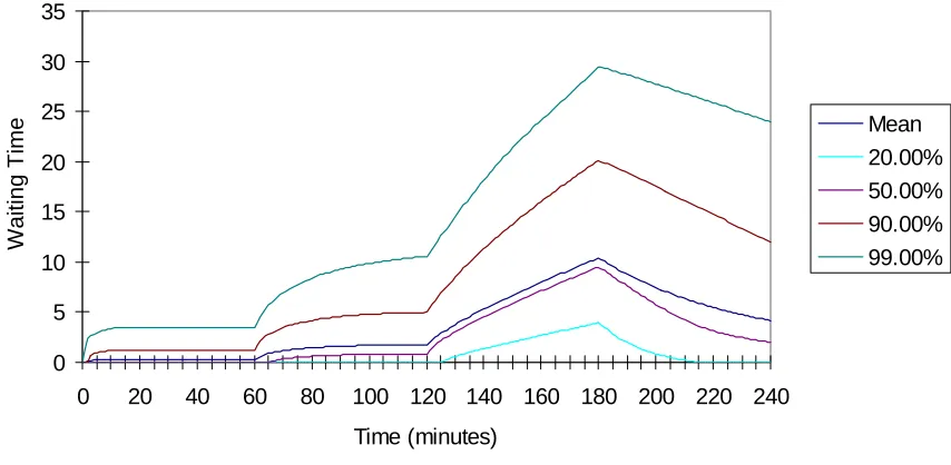
Figure 7: Performance Measures For First Cycle Where Traffic Intensity Exceeds 1 For 3rd Quarter

0 5 10 15 20 25 30 35

0 20 40 60 80 100 120 140 160 180 200 220 240 Time (minutes)

Waiting Time

Mean 20.00% 50.00% 90.00% 99.00%

8. Conclusions

An new exact model has been obtained for the time-dependent behaviour of virtual waiting time in discrete queueing systems of the form M(t)/G/c. However, in its full form, this model seriously inflates the computer time required to produce waiting time results over the time required to produce queue length results.

By introducing the Gamma family of distributions to approximate the conditional distribution of waiting time a highly accurate approximation has been developed that allows discrete time models for queue length to be extended to give virtual waiting time behaviour for very little extra computational effort.

Results presented demonstrate that the DTM approach has clear advantages compared with the SSA, PSA and MOL approaches in respect of time average performance measures. The advantages are even greater where time-dependent performance is important and where traffic intensities exceed one.

The accuracy of discrete time models of waiting time behaviour when applied to continuous time queues is yet to be investigated thoroughly, although the high accuracy of the DTM approach in estimating queue length behaviour gives reason for optimism.

Acknowledgements: The authors are very grateful for the suggestions and comments of the two anonymous referees, which led to improvements in the paper. In particular, we would like to acknowledge the contribution of one of the referees in improving our derivation of equations (13) and (14).

References

[2] Brahimi, M. and Worthington, D.J., “The finite capacity multi-server queue with inhomogeneous arrival rate and discrete service time distribution and its application to continuous service time problem,” Eur.J.Opl.Res.,50, 310-324, 1991.

[3] Choudhury, G., Lucantoni, D. and Whitt, W., “Multi-dimensional transform inversion with applications to the transient M/G/1 queue,” Report from AT&T Bell Laboratories, 1993.

[4] Cox D.R., “Renewal Theory”, Methuen & Co Ltd, page 64, 1962

[5] Dafermos, S. and Neuts, M.F., “A single server in discrete time,” Cahiers du Centre de Recherche Operationnelle, 13, 23-40, 1971.

[6] Eick, S.G., Massey, W.A. and Whitt, W., “M/G/∞ queues with sinusoidal arrival rates,” Mgmt.Sci.,39, 241-252, 1993.

[7] Frigui, I., Alfa, A.S., and Xu, X., “Algorithms for computing waiting time distributions under different queue disciplines for the D-BMAP/PH/1”, Naval Research Logistics, 44, 559-576, 1997.

[8] Green L. and Kolesar, P., “The lagged PSA for estimating peak congestion in multiserver Markovian queues with periodic arrival rates,” Mgmt.Sci., 43, 80-87, 1997.

[9] Green L. and Kolesar, P., “The pointwise stationary approximation for queues with nonstationary arrivals,” Mgmt.Sci., 37, 84-97, 1991.

[10] Green, L., Kolesar, P. and Soares, J., “Improving the SIPP approach for staffing service systems that have cyclic demands”, Opns.Res.,49, 549-564, 2001.

[11] Green, L., Kolesar, P. and Svoronos, S., “Some effects of nonstationarity on multi-server Markovian queueing systems”, Opns.Res.,39, 502-511, 1991.

[12] Gross, D. and Harris, C.M., Fundamentals of Queueing Theory, 3rd ed. John Wiley & Sons, New York, 1998.

[13] Jennings, O.B., Mandelbaum, A., Massey, W.A. and Whitt, W., “Server Staffing to meet Time-Varying Demand,” Mgmt.Sci., 42, 1383-1394, 1996.

[14] Meisling, T., “Discrete-Time Queueing Theory,” Operations Research,6, 96-105, 1958.

[15] Miller, A.C. and Rice, T.R., “Discrete approximations of probability distributions”, Mgmt.Sci., 29, 352-362, 1983.

[17] Neuts, M.F., “The single server queue in discrete time - numerical analysis 1,” Naval Res.Logist.Q.,20, 297-304, 1973.

[18] Omosigho, S.E. and Worthington, D.J., “An approximation of known accuracy for single server queues with inhomogeneous arrival rate and continuous service time distribution,” Eur.J.Opl.Res.,33, 304-313, 1988.

[19] Omosigho, S.E. and Worthington, D.J., “The single server queue with inhomogeneous arrival rate and discrete service time distribution,” Eur.J.Opl.Res.,22, 397-407, 1985.

[20] Sharma, O.P., Markovian Queues., Chichester: Ellis Horwood, 1990.

[21] Wall, A.D., Extending the scope of discrete time models to provide practical results for continuous time queueing systems, PhD Thesis, University of Lancaster, Lancaster, UK, 1995.

[22] Whitt W. “Approximating a Point Process by a Renewal Process, 1: Two Basic Methods”, Opns.Res.,30, 125-147, 1982.

[23] Whitt W. “Performance of the Queueing Network Analyzer”, Bell Sys.Tech.J., 62, 2817-2843, 1983. [24] Worthington, D.J. and Wall, A.D., “Using the Discrete Time Modelling Approach to Evaluate the

Time-Dependent Behaviour of Queueing Systems,” J Opl Res Soc,50, 777-788, 1999.