http://dx.doi.org/10.4236/jfrm.2016.51004
How to cite this paper: Slim, S. (2016). The Role of Trading Volume in Forecasting Market Risk. Journal of Financial Risk Management, 5, 22-34. http://dx.doi.org/10.4236/jfrm.2016.51004
The Role of Trading Volume in Forecasting
Market Risk
Skander Slim
Laboratory Research for Economy, Management and Quantitative Finance (LaREMFiQ), Institute of High Commercial Studies, University of Sousse, Sousse, Tunisia
Received 28 December 2015; accepted 8 March 2016; published 11 March 2016
Copyright © 2016 by author and Scientific Research Publishing Inc.
This work is licensed under the Creative Commons Attribution International License (CC BY). http://creativecommons.org/licenses/by/4.0/
Abstract
This paper examines the information content of trading volume in terms of forecasting the condi- tional volatility and market risk of international stock markets. The performance of parametric Value at Risk (VaR) models including the traditional RiskMetrics model and a heavy-tailed EGARCH model with and without trading volume is investigated during crisis and post-crisis pe- riods. Our empirical results provide compelling evidence that volatility forecasts based on vo- lume-augmented models cannot be outperformed by their competitors. Furthermore, our findings indicate that including trading volume into the volatility specification greatly enhances the perfor- mance of the proposed VaR models, especially during the crisis period. However, the volume effect is fairly overshadowed by the sufficient accuracy of the heavy-tailed EGARCH model, during the post-crisis period.
Keywords
Value at Risk, Risk Management, Trading Volume, EGARCH Model
1. Introduction
23
surrounding the volume-volatility relationship, we introduce trading volume into the model, particularly, within the EGARCH framework.
The investigation into the information content of trading volume will provide further insights into three relevant hypotheses currently upheld in the literature regarding the nature of the volume-volatility relation: the mixture of distributions hypothesis (MDH), the sequential information arrival hypothesis (SIH) and the noise trading hypothesis. Despite these distinctive assumptions, it is widely recognized that information flow is the key factor that underlies theories of the role of trading volume in explaining volatility and how information disseminates among market participants. The MDH predicts a positive contemporaneous volume-volatility relationship since the distribution of price change and volume is jointly subordinated to information flow (Clark, 1973; Epps & Epps, 1976; Harris, 1987; Tauchen & Pitts, 1983). Hence, past volume does not contain any additional useful information on the future dynamics of volatility. A number of empirical studies provide strong support to the MDH in stock markets (Chan & Fong, 1996; Jones et al., 1994; Karpoff, 1987; Lamoureux & La-strapes, 1990; Bollerslev & Jubinski, 1999; Giot et al., 2010; Slim & Dahmene, 2015, among others). In contrast, the SIH, proposed by Copeland (1976), and the noise trading hypothesis (Brock & LeBaron, 1996; Iori, 2002; Milton & Raviv, 1993) both suggest that a lead-lag (causal) relation exists, and hence, trading volume can be exploited for forecasting purpose.
Despite the considerable amount of research in this area, our special interest in the information content of trading volume in volatility forecasting rests on the scarcity of studies that use trading volume in an effort to improve the forceasting performance of VaR models. This line of research has not yet been pursued vigorously in the past, either because, in a risk management context, trading volume is typically employed to compute liquidity-adjusted VaR (Berkowitz, 2000; Almgren & Chriss, 2001; Subramanian & Jarrow, 2001; Angelidis & Benos, 2006, among others) or due the conflicting empirical evidence on the role of volume in forecasting vola-tility (Brooks, 1998; Wagner & Marsh, 2005). Besides Donaldson & Kamstra (2005) show that although lagged volume leads to no improvement in forecast performance, it does play an important switching role between the relative informativeness of ARCH and option implied volatility estimates. Fuertes et al. (2009) find limited forecast gains for lagged trading volume when it is incorporated into the GARCH modeling framework for assigning market conditions. Empirical evidence in compliance with the sequential information hypothesis saying that trading volume contains useful information of future return volatility is provided by Darrat et al. (2003) and Le & Zurbruegg (2010), among others.
In addition to the disagreements among previous studies on the empirical results, most of them evaluate volume-augmented volatility models only in terms of their forecasting ability, with little emphasis on examining the extend to which they may contribute to gauging and managing market risk. Therefore, other evaluation metrics and discussions on the applicability of trading volume as a risk management tool are needed to assess the practical usefulness of its information content. However, only a few studies have focused on this different dimension of the applicability of trading volume (Carchano et al., 2010; Asai & Brugal, 2013).
In this paper we empirically investigate the role of trading volume in predicting future volatility by comparing the relative performance of VaR forecasts generated by the EGARCH model versus both its volume-augmented counterparts and the traditional RiskMetrics model. We find some evidence of forecast improvement from the addition of trading volume, notecibly during periods of financial turmoil where statistical accuracy is hardly achieved by the investigated VaR models.
The remainder of the paper is organized as follows. Section 2 outlines the models and testing methodologies which are employed in the paper. The empirical results and a discussion of the findings are reported in Section 3. The final section provides a summary and conclusion.
2. Research Methodology
2.1. Volatility Models24
of conditional volatility in logarithmic form adds to the attractiveness of the model as it does not impose any positivity restrictions on the volatility coefficients. This property is practically appealing when exogenous variables are included into the volatility specification (Sucarrat & Escribano, 2012). The volatility models are described below (Models 1, 2, 3, and 4).
Mean equation: rt=µ σt+ t tz. (1) • Model 1: RiskMetrics
2 2 2
1 1
0.04 0.96 .
t zt t
σ = − + σ− (2)
• Model 2: EGARCH(1,1)
(
)
2 2
1 1 1 1
logσt = +ω α zt− −zt− +γzt− +βlogσt−. (3)
• Model 3: EGARCH(1,1) with detrended lagged volume (EGARCH-V)
(
)
2 2
1 1 1 1 1
logσt = +ω α zt− −zt− +γzt− +βlogσt− +δυt−. (4)
• Model 4: EGARCH(1,1) with lagged volume relative change (EGARCH-LV)
(
)
(
)
2 2
1 1 1 1 1 2
logσt = +ω α zt− −zt− +γzt− +βlogσt− +λlog Vt− Vt− . (5)
In the above equations, rt and σt denote the index return and its conditional volatility at time t, respec-
tivey. υt−1 denotes detrended log-volume and Vt−1 is the raw volume at time t−1. For the RiskMetrics model,
the innovation zt is distributed according to the standard normal distribution, whereas it is asumed to follow
the standardized skewed-t distribution in the remaning models. Following the parameterization provided by Laurent (2000), the probability density function of the standardized skewed-t is given by
(
)
(
)
(
)
2
| if ,
1
| ,
2
| if .
1
m
s g sz m z
s
f z
m
s g sz m z
s ξ ν ξ ξ ξ ν ξ ν ξ ξ
+ < −
+ = + ≥ − + (6)
where g
( )
. |ν is the symmetric (unit variance) Student’s-t density with ν degrees of freedom and ξ is theasymmetry parameter. In addition, m and 2
s are, respectively, the mean and the variance of the non- standardized skewed-t:
1 2 1 2 , π 2 m ν ν ξ ν ξ −
Γ −
= −
Γ
(7)
and
2 2 2
2 1
1 .
s ξ m
ξ
= + − −
(8)
It is straightforward to show that for the standardized skewed-t:
( )
(
)
2 1 2 4 2 , 1 π 1 2 z ν ν ξ ν ξ ν ξ + Γ −
=
+ − Γ
(9)
25 * , , , , . skst m skst s
α ν ξ α ν ξ
−
= (10)
where skstα ν ξ*, , denotes the quantile function of a non-standardized skewed-t distribution (Lambert & Laurent,
2000):
(
)
(
)
2 , 2 * , , 2 , 2 1 1 1 if 2 1 1 1 1 if 2 1 st skst st α ν α ν ξα ν
α ξ α
ξ ξ
α
ξ ξ α
ξ
−
+ <
+ = − − + ≥ + (11)
where stα ν, is the quantile function of the (unit variance) Student’s-t distribution.
2.2. Volatility Forecast Evaluation
Forecast evaluations are a key component of empirical studies that use time series because good forecasts are valuable for decision making. A model is said to be superior to another model if it provides more accurate forecasts. We use the Superior Predictive Ability (SPA) test, introduced by Hansen (2005), to gauge the one-day-ahead forecasting accuracy of the four competing models.1 The SPA test enables the comparison of the performance of a benchmark forecasting model simultaneously to that of a whole set of competitors under a specific loss function. The null hypothesis of the test is that the benchmark model is not outperformed by all alternative models. The SPA test is performed by using the mean squared-error (MSE) and the quasi-likelihood (QLIKE) loss functions. These loss functions are robust to noisy proxies for the true unobserved volatility as proved by Patton (2011). The MSE and the QLIKE are defined, respectively, as
(
2 2)
1 1 , T t t t MSE RVT = σ
=
∑
− (12)2 2 2 2 1 1 log 1. T t t
t t t
RV RV
QLIKE
T = σ σ
=
∑
− − (13)where T is the number of forecasting data points. RVt2 and
2
t
σ refer to the realized (actual) variance and the variance forecast from a particular model, repectively. The proxy this paper uses for realized variance is the squared-returns.
2.3. VaR Framework and Backtesting
The VaR estimate of the portfolio at level α for a time horizon of k-days at time t indicates the loss of the portfolio over k-days at time t that is exceeded with a small target probability α such that;
, | .
t k t k t
Prob r + < −VaR+ α =α (14)
where rt k+ denotes the return from time t to time t+k, and t is the information set at time t. From the
daily volatility forecast, the one-day VaR estimate for a long trading position at time t is given by
( )
1, ˆ .1
t t
VaR+α =qα z σ+ (15)
where qα
( )
z denotes the quantile implied by the probability distribution of the return innovations at theprobability level α and σˆt+1 is the one-day-ahead volatility forecast at time t.
To measure the performance of the VaR models, we backtest the VaR estimates with the realized losses using the unconditional coverage criterion developed by Kupiec (1995) and the conditional coverage test of Christof-fersen (1998). Backtesting is a formal statistical framework that consists in verifying if actual trading losses are in line with model-generated VaR forecasts, and relies on testing over VaR violations (also called the hit). A
1The SPA test is more robust than similar approaches, such as reality check test (White, 2000) or tests for equal predictive ability (Diebold &
26
violation is said to occur when the realized loss exceeds the VaR threshold. The Unconditional Coverage (UC) test has been established as an the industry standard mostly due to the fact that it is implicitly incorporated in the “traffic Light” system proposed by the Basel Committee on Banking Supervision (2006, 2009), which remains the reference backtest methodology for banking regulators. The test consists of examining if the proportion of violations (failures) is equal to the expected one. This is equivalent to testing if the hit variable It
( )
α , whichtakes values of 1 if the loss exceeds the reported VaR measure and 0 otherwise, follows a binomial distribution with parameter α . Under the UC hypothesis, the likelihood ratio (LR) test statistic follows a χ2 distribution with one degree of freedom. That is:
( )
(
)
( ) ( )
ˆ ˆ 2( )
2 ln 1 T N N 2 ln 1 T N N ~ 1 .
UC
LR α = − −α − α + − f − f χ
(16)
where ˆf =N T is the empirical failure rate and N is the number of days over a period T that a violation has occurred.
An enhancement of the unconditional backtesting framework is achieved by additionally testing for the independence (IND) of the sequence of VaR violations yielding a combined test of Conditional Coverage (CC). The Christoffersen’s (1998) CC test involves the estimation of the following statistic:
( )
( )
( )
2( )
~ 2 .
CC UC IND
LR α =LR α +LR α χ (17)
where LRIND denotes the LR test for independence, against an explicit first-order Markov alternative, which is
given by
( )
(
)
(
)
00 01(
)
10 11 2( )
01 01 11 11
ˆ ˆ ˆ ˆ
2 ln 1 T N N 2 ln 1 n n 1 n n ~ 1 .
IND
LR α = − −α − α + −π π −π π χ (18)
where nij; i j, =0,1 is the number of times we have It
( )
α = j and It−1( )
α =i with πˆ01=n01(
n00+n01)
and πˆ11=n11
(
n10+n11)
.3. Empirical Findings
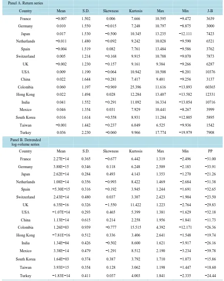
3.1. DataThe dataset refer to two groups of stock market indices, namely developed and emerging, covering the geogra- phical regions of Asia, Latin America and Europe. Specifically, the following stock market indices are used: France (CAC 40); Germany (GDAX); Japan (NIKKEI225); Netherlands (AEX); Spain (IBEX35); Switzerland (SSMI); UK (FTSE100); USA (DJIA); China (SSE Composite); Colombia (CSE ALL-SHARE); Hong Kong (HSI); India (NSEI); Mexico (IPC); South Korea (KOSPI Composite); Taiwan (TWSE) and Turkey (BIST100). Daily closing prices and raw trading volumes are obtained from Thomson Reuters Eikon for the period between January 2000 and September 2015, yielding a total of 4014 observations for each stock market. Table 1reports descriptive statistics for daily returns, estimated on a continuously compounded basis, and detrended log-volume series, respectively.2 These summary statistics reveal the usual characteristics of financial returns, namely a mean value which is dominated by the standard deviation value and evidence of non-normality. Most of the returns series are negatively skewed (12 out of 16 markets) as illustrated byTable 1. The unit root test confirms that the detrended volume series are stationary.
3.2. SPA Test Results
We begin by evaluating the forecasting performance of the four volatility models presented in 2.1. We use a rolling window that includes eight years of historical records to derive recursive one-day-ahead volatility forecasts. The rolling window technique updates the estimation sample regularly by incorporating new information reflected in each sample of daily returns and trading volumes. All the models are updated on a monthly basis, and the forecasting performance is assessed over the out of-sample period from August 1, 2007
2As pointed out by Gallant et al. (1992), there is significant evidence of both linear and nonlinear time trends in the trading volume series.
Therefore, we run the following regression: 2
0 1 2
logVt=a +a t+a t +υt, where Vt denotes the raw volume and the residual υt stands for
27
Table 1. Summary statistics.
Panel A. Return series
Country Mean S.D. Skewness Kurtosis Max Min J-B
France −0.007 1.502 0.006 7.666 10.595 −9.472 3639
Germany 0.010 1.550 −0.015 7.248 10.797 −8.875 3000
Japan 0.017 1.530 −0.500 10.345 13.235 −12.111 7423
Netherlands −0.011 1.480 −0.092 9.242 10.028 −9.590 6521
Spain −0.004 1.519 0.082 7.761 13.484 −9.586 3762
Switzerland 0.005 1.214 −0.168 9.915 10.788 −9.070 7873
UK −0.002 1.230 −0.157 9.161 9.384 −9.266 6287
USA 0.009 1.190 −0.064 10.942 10.508 −8.201 10376
China 0.022 1.644 −0.281 7.417 9.401 −9.256 3137
Colombia 0.060 1.197 −0.969 25.396 11.616 −13.893 60365
Hong Kong 0.022 1.494 0.028 12.284 13.407 −13.582 12331
India 0.041 1.552 −0.291 11.092 16.334 −13.054 10716
Mexico 0.046 1.354 0.031 7.929 10.441 −8.267 3999
South Korea 0.016 1.614 −0.558 8.931 11.284 −12.805 5895
Taiwan −0.001 1.442 −0.237 6.049 6.525 −9.936 1542
Turkey 0.036 2.230 −0.060 9.966 17.774 −19.979 7908
Panel B. Detrended log-volume series
Country Mean S.D. Skewness Kurtosis Max Min PP
France 2.27E−14 0.365 −0.677 6.442 1.319 −2.496 −31.00
Germany 3.88E−15 0.346 0.118 6.248 2.509 −2.183 −33.91
Japan 2.62E−14 0.284 0.493 4.143 1.353 −1.270 −21.26
Netherlands 1.08E−14 0.356 −0.993 8.422 1.469 −2.684 −31.38
Spain −5.30E−15 0.316 −0.192 3.945 1.244 −1.691 −32.65
Switzerland 2.43E−14 0.480 0.037 3.307 2.423 −1.904 −23.50
UK 6.35E−16 0.326 −1.550 11.422 1.223 −2.764 −29.83
USA −1.07E−14 0.293 0.465 5.399 1.381 −1.629 −32.18
China 1.13E−14 0.615 0.214 2.258 1.956 −1.841 −11.73
Colombia 1.26E−03 0.939 −0.777 15.515 4.392 −12.171 −26.36
Hong Kong −7.81E−16 0.512 0.336 3.406 2.641 −1.548 −19.74
India 1.34E−04 0.426 −0.502 8.600 1.621 −3.917 −26.16
Mexico 3.38E−14 0.479 −1.291 8.512 2.190 −3.234 −39.78
South Korea 1.64E−03 0.374 0.387 3.792 1.710 −1.073 −15.86
Taiwan 3.93E−15 0.354 0.128 3.062 1.198 −1.447 −18.60
Turkey −1.83E−14 0.411 0.037 4.003 1.841 −2.335 −24.44
This table reports descriptive statistics of scaled [100×] daily logarithmic index returns (Panel A) and detrended log-volume series (Panel B). S.D.,
Min and Max are the standard deviation, the minimum and maximum values of the sample data, respectively. Skewness and Kurtosis are the
estimated centralized third and fourth moments of the data. J-B isthe Jarque & Bera (1980) test for normality ( 2( )
2
χ distributed). The PP statistic is
28
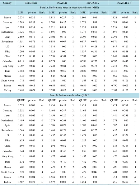
to Spetember 10, 2015. We then compare their forecasting performance by using the two mean loss functions (MSE and QLIKE). A forecasting model with the smallest loss function value does not imply the superiority of that model among its competitors (Hansen & Lunde, 2005). Such a conclusion cannot be made on the basis of just one criterion and just one sample. For this reason, all the models considered in this study are consecutively taken as benchmark models in order to evaluate whether a particular model (benchmark) is significantly outperformed by other competing models using the SPA test. The p-values of the test are computed using the stationary bootstrap of Politis & Romano (1994) generating 10,000 bootstrap re-samples. A high p-value indi- cates that the benchmark model is not outperformed by the competing models.
The resuts reported inTable 2 show that the RiskMetrics model is dominated by the heavy-tailed EGARCH model with and without trading volume for most of the markets whatever the loss function considered. However, regarding the MSE criteria, we can see that none of the EGARCH specifications is found to absolutely outperform the others across markets. The EGARCH is the best performing model for Netherlands, UK, USA, Colombia and South Africa. The EGARCH-V is selected for France, Germany, China, Mexico, Taiwan and Turkey while the EGARCH-LV is selected for the remaining markets (i.e., Japan, Sapin, Switzerlands, Hong Kong and India). Although, the results highlight the superiority of volume-augmented models for 11 out of 16 markets, it is not clear which measure of trading volume would likely lead to gains in forecasting accuracy. The asymmetric QLIKE loss function provides further insights into the role of trading volume in volatility fore- casting. According to the QLIKE criteria, the volume-augmented models are selected for all the markets except South Africa. FromTable 2, Panel B., we can see that the best performing model is the EGARCH-V for 12 out of 16 markets followed by the EGARCH-LV model which yields in 3 out of 16 cases the lowest forecasing error.
Unlike the MSE criteria, the asymmetric QLIKE loss function suggests that the introduction of trading volume level into the EGARCH equation leads to a significant improvement of the out-of-sample volatility estimations relative to trading volume variations. This finding has important implications for risk management since the QLIKE more heavily penalizes under-perdiction than over-prediction and it also reduces the effect of heteroskedasticity by scaling forecasting errors with actual volatilities (Bollerslev & Ghysels, 1996). Ac- cordingly, the economic value of forecast accuracy provided by the EGARCH-V model is sufficiently higher than its competitors as they are likely to under-predict future volatility which is costly compared to over- perdiction, especially during maket meltdowns (Taylor, 2014).
3.3. VaR Peformance
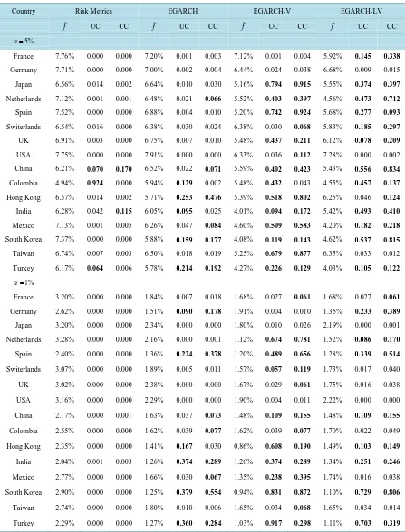
Using the out-of-sample volatility forecasts described in Section 3.2, we calculate and evaluate the one-day VaR estimates based on the UC and CC tests. To investigate the ability of the VaR models into measuring the risk with sufficient accuracy in different volatility scenarios, we split the evaluation sample into two sub-samples. The first forecast period starts on August 1, 2007 to include the sub-prime financial crisis (Covitz et al., 2013). The second forecast period is referred to as the post-crisis period from May 15, 2012 to September 10, 2015.
Table 3and Table 4 are constructed in the same manner and report the empirical failure rate, the UC and CC
test results during crisis and post-crisis periods, respectively. The results in Table 3 suggest that the EGARCH model outperforms the RiskMetrics model, although it provides a partial improvement to the model for estimating the VaR. The volume-augmented EGARCH models provide substantial improvement and exhibit fairly equivalent statistical accuracy for the 5% VaR. For the 1% VaR, the best performing model is the EGARCH-V followed by the EGARCH-LV. Interestingly, the performance of the EGARCH-V model improves considerably by providing correct conditional coverage for 13 out of 16 markets (nearly 80% of the sample), compared to the EGARCH model which exhibits a conditional coverage acceptance rate of 50% amongest the examined markets. This finding suggests that risk managers may profit from expanding the traditional ARCH information set to include volume measures, in addition to the history of lagged return innovations.
29
Table 2. SPA test results of volatility models.
Country RiskMetrics EGARCH EGARCH-V EGARCH-LV
Panel A. Performance based on mean squared error (MSE)
MSE p-value Rank MSE p-value Rank MSE p-value Rank MSE p-value Rank
France 2.034 0.032 4 1.813 0.227 2 1.806 1.000 1 1.826 0.067 3
Germany 1.763 0.053 4 1.580 0.457 2 1.575 1.000 1 1.583 0.068 3
Japan 3.188 0.039 4 2.821 0.059 3 2.820 0.088 2 2.756 1.000 1
Netherlands 1.926 0.037 4 1.695 1.000 1 1.719 0.089 3 1.695 0.645 1
Spain 2.609 0.010 4 2.402 0.111 3 2.398 0.049 2 2.390 1.000 1
Switerlands 1.051 0.071 4 0.886 0.067 2 0.887 0.071 3 0.871 1.000 1
UK 1.149 0.022 4 1.016 1.000 1 1.017 0.428 2 1.017 0.120 3
USA 1.200 0.063 4 1.028 1.000 1 1.037 0.531 3 1.033 0.888 2
China 2.822 0.181 3 2.796 0.384 2 2.783 1.000 1 2.841 0.034 4
Colombia 0.816 0.040 4 0.779 1.000 1 0.786 0.275 3 0.782 0.492 2
Hong Kong 3.707 0.042 4 3.240 0.041 3 3.226 0.373 2 3.212 1.000 1
India 3.188 0.042 4 2.820 0.057 2 2.820 0.085 2 2.756 1.000 1
Mexico 1.145 0.035 4 1.047 0.261 2 1.039 1.000 1 1.062 0.299 3
South Korea 1.716 0.037 4 1.546 1.000 1 1.565 0.120 3 1.564 0.106 2
Taiwan 0.654 0.015 3 0.639 0.030 2 0.634 1.000 1 0.790 0.003 4
Turkey 2.631 0.029 3 2.748 0.012 4 2.534 1.000 1 2.537 0.103 2
Panel B. Performance based on QLIKE
QLIKE p-value Rank QLIKE p-value Rank QLIKE p-value Rank QLIKE p-value Rank
France 1.529 0.000 4 1.430 0.455 3 1.428 1.000 1 1.429 0.531 2
Germany 1.552 0.004 4 1.466 0.247 2 1.464 1.000 1 1.466 0.201 2
Japan 1.532 0.002 4 1.450 0.120 3 1.432 1.000 1 1.441 0.291 2
Netherlands 1.499 0.000 4 1.379 0.298 2 1.400 0.000 3 1.378 1.000 1
Spain 1.481 0.000 4 1.386 0.071 3 1.385 0.066 2 1.382 1.000 1
Switerlands 1.566 0.000 4 1.463 0.178 3 1.461 0.272 2 1.457 1.000 1
UK 1.513 0.000 4 1.432 0.352 2 1.429 1.000 1 1.432 0.379 2
USA 1.629 0.000 4 1.546 0.003 3 1.525 1.000 1 1.533 0.071 2
China 1.595 0.069 4 1.594 0.032 3 1.576 1.000 1 1.583 0.364 2
Colombia 1.749 0.000 4 1.639 0.355 2 1.636 1.000 1 1.650 0.082 3
Hong Kong 1.511 0.001 4 1.472 0.008 3 1.455 1.000 1 1.470 0.018 2
India 1.532 0.003 4 1.450 0.119 3 1.432 1.000 1 1.441 0.289 2
Mexico 1.488 0.002 3 1.428 0.123 2 1.424 1.000 1 1.496 0.000 4
South Korea 1.521 0.002 4 1.468 1.000 1 1.479 0.042 2 1.481 0.016 3
Taiwan 1.558 0.004 3 1.524 0.023 2 1.516 1.000 1 1.750 0.000 4
Turkey 1.507 0.029 3 1.579 0.000 4 1.454 1.000 1 1.455 0.437 2
This table reports the mean losses of the different volatility models over the out-of-sample period (August 2007-September 2015) with respect to two
evaluation criteria (MSE × 10−6 and QLIKE). Models in each panel are sorted according to the consistent version of the SPA test under the selected
30
Table 3. VaR forecasting performance during the crisis period.
Country Risk Metrics EGARCH EGARCH-V EGARCH-LV
ˆ
f UC CC fˆ UC CC fˆ UC CC fˆ UC CC
5%
α=
France 7.76% 0.000 0.000 7.20% 0.001 0.003 7.12% 0.001 0.004 5.92% 0.145 0.338
Germany 7.71% 0.000 0.000 7.00% 0.002 0.004 6.44% 0.024 0.038 6.68% 0.009 0.015
Japan 6.56% 0.014 0.002 6.64% 0.010 0.030 5.16% 0.794 0.915 5.55% 0.374 0.397
Netherlands 7.12% 0.001 0.001 6.48% 0.021 0.066 5.52% 0.403 0.397 4.56% 0.473 0.712
Spain 7.52% 0.000 0.000 6.88% 0.004 0.010 5.20% 0.742 0.924 5.68% 0.277 0.093
Switerlands 6.54% 0.016 0.000 6.38% 0.030 0.024 6.38% 0.030 0.068 5.83% 0.185 0.297
UK 6.91% 0.003 0.000 6.75% 0.007 0.010 5.48% 0.437 0.211 6.12% 0.078 0.209
USA 7.75% 0.000 0.000 7.91% 0.000 0.000 6.33% 0.036 0.112 7.28% 0.000 0.002
China 6.21% 0.070 0.170 6.52% 0.022 0.071 5.59% 0.402 0.423 5.43% 0.556 0.834
Colombia 4.94% 0.924 0.000 5.94% 0.129 0.002 5.48% 0.432 0.043 4.55% 0.457 0.137
Hong Kong 6.57% 0.014 0.002 5.71% 0.253 0.476 5.39% 0.518 0.802 6.25% 0.046 0.124
India 6.28% 0.042 0.115 6.05% 0.095 0.025 4.01% 0.094 0.172 5.42% 0.493 0.410
Mexico 7.13% 0.001 0.005 6.26% 0.047 0.084 4.60% 0.509 0.583 4.20% 0.182 0.218
South Korea 7.37% 0.000 0.000 5.88% 0.159 0.177 4.08% 0.119 0.143 4.62% 0.537 0.815
Taiwan 6.74% 0.007 0.003 6.50% 0.018 0.019 5.25% 0.679 0.877 6.35% 0.033 0.012
Turkey 6.17% 0.064 0.006 5.78% 0.214 0.192 4.27% 0.226 0.129 4.03% 0.105 0.122
1%
α=
France 3.20% 0.000 0.000 1.84% 0.007 0.018 1.68% 0.027 0.061 1.68% 0.027 0.061
Germany 2.62% 0.000 0.000 1.51% 0.090 0.178 1.91% 0.004 0.010 1.35% 0.233 0.389
Japan 3.20% 0.000 0.000 2.34% 0.000 0.000 1.80% 0.010 0.026 2.19% 0.000 0.001
Netherlands 3.28% 0.000 0.000 2.16% 0.000 0.001 1.12% 0.674 0.781 1.52% 0.086 0.170
Spain 2.40% 0.000 0.000 1.36% 0.224 0.378 1.20% 0.489 0.656 1.28% 0.339 0.514
Switerlands 3.07% 0.000 0.000 1.89% 0.005 0.011 1.57% 0.057 0.119 1.73% 0.017 0.040
UK 3.02% 0.000 0.000 2.38% 0.000 0.000 1.67% 0.029 0.061 1.75% 0.016 0.038
USA 3.16% 0.000 0.000 2.29% 0.000 0.000 1.90% 0.004 0.011 2.22% 0.000 0.000
China 2.17% 0.000 0.001 1.63% 0.037 0.073 1.48% 0.109 0.155 1.48% 0.109 0.155
Colombia 2.55% 0.000 0.000 1.62% 0.039 0.077 1.62% 0.039 0.077 1.70% 0.022 0.049
Hong Kong 2.35% 0.000 0.000 1.41% 0.167 0.030 0.86% 0.608 0.190 1.49% 0.103 0.149
India 2.04% 0.001 0.003 1.26% 0.374 0.289 1.26% 0.374 0.289 1.34% 0.251 0.246
Mexico 2.77% 0.000 0.000 1.66% 0.030 0.067 1.35% 0.238 0.395 1.74% 0.016 0.038
South Korea 2.90% 0.000 0.000 1.25% 0.379 0.554 0.94% 0.831 0.872 1.10% 0.729 0.806
Taiwan 2.74% 0.000 0.000 1.80% 0.010 0.006 1.65% 0.034 0.068 1.65% 0.034 0.014
Turkey 2.29% 0.000 0.000 1.27% 0.360 0.284 1.03% 0.917 0.298 1.11% 0.703 0.319
This table reports the VaR results during the crisis period (August 2007-May 2012). ˆf denotes the empirical failure rate for each model, UC is the
p-value for the unconditional coverage test, and CC is the p-value for the conditional coverage test. Bold numbers indicate significance at the 5%
31
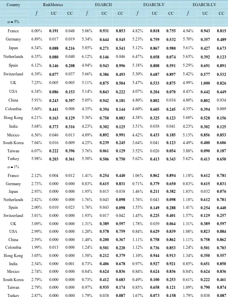
Table 4. VaR forecasting performance during the post-crisis period.
Country RiskMetrics EGARCH EGARCH-V EGARCH-LV
ˆ
f UC CC fˆ UC CC fˆ UC CC fˆ UC CC
5%
α=
France 6.00% 0.191 0.048 5.06% 0.931 0.853 4.82% 0.818 0.755 4.94% 0.943 0.815
Germany 6.89% 0.017 0.019 5.34% 0.644 0.545 5.23% 0.759 0.532 5.70% 0.357 0.489
Japan 6.34% 0.088 0.216 5.85% 0.271 0.541 5.12% 0.867 0.980 5.61% 0.427 0.673
Netherlands 6.35% 0.080 0.040 6.12% 0.146 0.046 6.47% 0.058 0.074 5.65% 0.392 0.123
Spain 6.12% 0.146 0.208 4.94% 0.943 0.996 5.18% 0.808 0.591 5.29% 0.691 0.891
Switzerland 6.39% 0.077 0.037 5.66% 0.386 0.493 5.30% 0.687 0.897 5.42% 0.577 0.532
UK 7.25% 0.005 0.005 5.11% 0.875 0.504 5.47% 0.533 0.875 4.99% 1.000 0.826
USA 6.34% 0.086 0.153 5.14% 0.843 0.222 4.07% 0.204 0.070 4.43% 0.442 0.449
China 5.91% 0.243 0.397 5.05% 0.942 0.181 4.80% 0.802 0.034 4.80% 0.802 0.034
Colombia 5.60% 0.441 0.008 4.35% 0.394 0.144 4.60% 0.605 0.245 4.35% 0.394 0.009
Hong Kong 6.21% 0.163 0.129 5.36% 0.750 0.083 4.38% 0.325 0.123 5.60% 0.528 0.156
India 5.68% 0.373 0.316 4.23% 0.302 0.125 3.51% 0.038 0.041 4.23% 0.302 0.125
Mexico 6.56% 0.046 0.013 4.89% 0.892 0.991 4.42% 0.433 0.185 5.13% 0.856 0.853
South Korea 7.04% 0.016 0.009 4.25% 0.239 0.245 3.64% 0.041 0.123 4.49% 0.400 0.606
Taiwan 6.07% 0.222 0.396 3.76% 0.061 0.129 3.52% 0.026 0.054 3.88% 0.090 0.187
Turkey 5.98% 0.203 0.361 5.50% 0.506 0.750 5.62% 0.413 0.343 5.62% 0.413 0.650
1%
α=
France 2.12% 0.004 0.012 1.41% 0.254 0.440 1.06% 0.862 0.894 1.18% 0.612 0.781
Germany 2.73% 0.000 0.000 0.83% 0.615 0.831 0.71% 0.379 0.650 0.83% 0.615 0.831
Japan 2.93% 0.000 0.000 1.95% 0.015 0.038 1.46% 0.211 0.382 1.83% 0.032 0.076
Netherlands 2.82% 0.000 0.000 1.76% 0.043 0.098 1.76% 0.043 0.098 1.18% 0.612 0.781
Spain 2.00% 0.010 0.023 1.76% 0.043 0.098 1.53% 0.149 0.288 1.41% 0.254 0.440
Switzerland 3.01% 0.000 0.000 1.93% 0.017 0.042 1.45% 0.225 0.401 1.57% 0.129 0.257
UK 3.09% 0.000 0.000 1.31% 0.389 0.597 1.78% 0.039 0.064 1.31% 0.389 0.597
USA 2.99% 0.000 0.000 1.20% 0.578 0.759 0.84% 0.629 0.839 1.08% 0.823 0.884
China 2.59% 0.000 0.000 1.48% 0.200 0.367 1.11% 0.758 0.862 1.11% 0.758 0.862
Colombia 1.99% 0.013 0.000 1.24% 0.501 0.220 1.12% 0.736 0.853 1.24% 0.501 0.703
Hong Kong 3.05% 0.000 0.000 1.58% 0.212 0.379 1.10% 0.944 0.913 1.34% 0.350 0.557
India 2.54% 0.000 0.001 0.73% 0.406 0.678 0.97% 0.927 0.921 0.85% 0.651 0.850
Mexico 2.74% 0.000 0.000 0.84% 0.624 0.836 0.84% 0.624 0.836 0.84% 0.624 0.836
South Korea 2.79% 0.000 0.000 0.73% 0.412 0.683 0.49% 0.100 0.253 0.61% 0.222 0.461
Taiwan 2.79% 0.000 0.000 0.97% 0.935 0.174 0.85% 0.658 0.121 1.09% 0.790 0.874
Turkey 2.87% 0.000 0.000 1.79% 0.038 0.087 1.67% 0.073 0.158 1.79% 0.038 0.087
This table reports the VaR results during the post-crisis period (May 2012-September 2015). ˆf denotes the empirical failure rate for each model,
UC is the p-value for the unconditional coverage test, and CC is the p-value for the conditional coverage test. Bold numbers indicate significance at
32
both 1% and 5% loss quantiles seem to be more predictable, during the post-crisis period, as statistical sufficiency is achieved effortlessly by the three non-normal EGARCH models for most of the investigated markets. For the 5% VaR, Both the EGARCH and EGARCH-LV models perform exceptionally well. The hypothesis of correct unconditional coverage cannot be rejected for all the markets while it is rejected for the EGARCH-V in the case of 3 markets (i.e., India, South Korea and Taiwan). Regarding the CC test, the three EGARCH models provide almost equal statistical accuracy. Besides, we find slight improvement from the addition of trading volume for 1% VaR. Indeed, the EGARCH model exhibits higher rejection rates (5 and 2 out of 16 markets regarding the UC and CC tests, respectively) compared to both EGARCH-V and EGARCH-LV for which VaR accuracy cannot be rejected by the CC test for all the markets while it is rejected only in the case of 2 markets, according to the UC test.
4. Conclusion
Using a long data sample of developed and emerging stock market indices, this article examines the relevance and usefulness of trading volume in forecasting the conditional volatility and market risk. Specifically, this study empirically investigates the one-day-ahead forecasting performance of volume-augmented volatility models by employing two consistent loss functions casted into the SPA test, and two backtesting procedures (i.e., uncon- ditional and conditional coverage tests). Hence, our empirical framework allows to not only test the information content of trading volume in forecasting the return volatility as it has been done in several past studies (e.g. Brooks, 1998; Wagner & Marsh, 2005; Fuertes et al., 2009; Le & Zurbruegg, 2010), but also to investigate its suitability as an additional information variable in terms of quantifying market risk (VaR) as well as the stability of the VaR estimates during high volatility period (crisis) and market calm (post-crisis).
The empirical results are quite interesting and offer many implications. Despite the claimed different attributes of emerging compared to developed equity markets, the most successful models are common in both asset classes. Our overall results lead to the overwhelming conclusion that the skewed-t EGARCH model outperforms the RiskMetrics model. This finding supports earlier evidence that models which include asymmetric and heavy-tailed distributions perform substantially better than those with normal innovations. Besides, we find that the accuracy of the one-day-ahead VaR forecasts can be significantly improved by accounting for the volume effect, in particular, during market meltdowns and most markedly by introducing lagged trading volume into the EGARCH model rather than lagged trading volume relative change. However, the information content of trading volume is overshadowed in the low volatility state where the heavy-tailed EGARCH model and its two augmented counterparts appear to be remarkably accurate, providing almost equal statistical sufficiency.
In light of the promising results provided by the trade size, one may consider the number of trades as an alternative measure of trading volume. Hence, based on the hypothesis that the number of trades is the main driving force behind the volume-volatility relationship (Chordia & Subrahmanyam, 2004; Foster & Viswanathan, 1996; Kyle, 1985), a thorough investigation of the its effectiveness as an instrument of risk management will be an interesting avenue for further research.
References
Almgren, R., & Chriss, N. (2001). Optimal Execution of Portfolio Transactions. Journal of Risk, 3, 5-39.
Angelidis, T., & Benos, A. (2006). Liquidity Adjusted Value-at-Risk Based on the Components of the Bid-Ask Spread. Ap-plied Financial Economics, 16, 835-851. http://dx.doi.org/10.1080/09603100500426440
Asai, M., & Brugal, I. (2013). Forecasting Volatility via Stock Return, Range, Trading Volume and Spillover Effects: The Case of Brazil. North American Journal of Economics and Finance, 25, 202-213.
http://dx.doi.org/10.1016/j.najef.2012.06.005
Basel Committee on Banking Supervision (2006). Basel II: International Convergence of Capital Measurement and Capital Standards: A Revised Framework. Technical Report, Bank for International Settlements, Basel, Switzerland.
Basel Committee on Banking Supervision (2009). Revisions to the Basel II Market Risk Framework: Final Version. Tech-nical Report, Bank for International Settlements, Basel, Switzerland.
33
Bollerslev, T. (1986). Generalized Autoregressive Conditional Heteroskedasticty. Journal of Econometrics, 31, 307-327.
http://dx.doi.org/10.1016/0304-4076(86)90063-1
Bollerslev, T., & Ghysels, E. (1996). Periodic Autoregressive Conditional Heteroscedasticity. Journal of Business and Eco-nomic Statistics, 14, 139-151.
Bollerslev, T., & Jubinski, D. (1999). Equity Trading Volume and Volatility: Latent Information Arrivals and Common Long-Run Dependencies. Journal of Business and Economics Statistics, 17, 9-21.
Brock, W. A., & LeBaron, B. D. (1996). A Dynamic Structural Model for Stock Return Volatility and Trading Volume. Re-view of Economics and Statistics, 78, 94-110. http://dx.doi.org/10.2307/2109850
Brooks, C. (1998). Predicting Stock Index Volatility: Can Market Volume Help? Journal of Forecasting, 17, 59-80.
http://dx.doi.org/10.1002/(SICI)1099-131X(199801)17:1<59::AID-FOR676>3.0.CO;2-H
Carchano, O., Rachev, S., Sung, W., & Kim, A. (2010). Volume Adjusted VaR in Spot and Futures Markets. Technical Re-port, Stony Brook, NY: Stony Brook University.
Chan, K. and Fong, W. (1996). Realized Volatility and Transactions. Journal of Banking and Finance, 30, 2063-2085.
http://dx.doi.org/10.1016/j.jbankfin.2005.05.021
Chordia, T., & Subrahmanyam, A. (2004). Order Imbalance and Individual Stock Returns: Theory and Evidence. Journal of Financial Economics, 72, 485-518. http://dx.doi.org/10.1016/S0304-405X(03)00175-2
Christoffersen, P. (1998). Evaluating Interval Forecasts. International Economic Review, 39, 841-862.
http://dx.doi.org/10.2307/2527341
Clark, P. K. (1973). A Subordinated Stochastic Process Model with Finite Variance for Speculative Process. Econometrica, 41, 135-155. http://dx.doi.org/10.2307/1913889
Copeland, T. E. (1976). A Model of Asset Trading under the Assumption of Sequential Information Arrival. Journal of Finance, 34, 1149-1168. http://dx.doi.org/10.2307/1913889
Covitz, D., Liang, N., & Suarez, G. A. (2013). The Evolution of a Financial Crisis: Collapse of the Asset-Backed Commer-cial Paper Market. Journal of Finance, 68, 815-848. http://dx.doi.org/10.1111/jofi.12023
Darrat, A., Rahman, S., & Zhong, M. (2003). Intraday Trading Volume and Return Volatility of the DJIA Stocks: A Note. Journal of Banking and Finance, 27, 2035-2043. http://dx.doi.org/10.1016/S0378-4266(02)00321-7
Diebold, F., & Mariano, R. (1995). Comparing Predictive Accuracy. Journal of Business and Economic Statistics, 13, 253- 263.
Donaldson, G., & Kamstra, M. (2005). Volatility Forecasts, Trading Volume, and the Arch versus Option-Implied Volatility Trade-Off. Journal of Financial Research, 28, 519-538. http://dx.doi.org/10.1111/j.1475-6803.2005.00137.x
Engle, R. (1982). Autoregressive Conditional Heteroskedasticity with Estimates of the Variance with Estimates of the Va-riance of United Kingdom Inflation. Econometrica, 50, 987-1007. http://dx.doi.org/10.2307/1912773
Epps, T. W., & Epps, M. L. (1976). The Stochastic Dependence of Security Price Changes and Transaction Volumes: Impli-cations for the Mixture-of-Distribution Hypothesis. Econometrica, 44, 305-321. http://dx.doi.org/10.2307/1912726
Foster, F., & Viswanathan, S. (1996). Strategic Trading When Agents Forecast the Forecasts of Others. Journal of Finance, 51, 1437-1478. http://dx.doi.org/10.1111/j.1540-6261.1996.tb04075.x
Fuertes, A. M., Izzeldin, M., & Kalotychou, E. (2009). On Forecasting Daily Stock Volatility: The Role of Intraday Informa-tion and Market CondiInforma-tions. International Journal of Forecasting, 25, 259-281.
http://dx.doi.org/10.1016/j.ijforecast.2009.01.006
Gallant, A. R., Rossi, P. E., & Tauchen, G. (1992). Stock Prices and Volumes. Review of Financial Studies, 5, 199-242.
http://dx.doi.org/10.1093/rfs/5.2.199
Giot, P., Laurent, S., & Petitijean, M. (2010). Trading Activity, Realized Volatility and Jumps. Journal of Empirical Finance, 17, 168-175. http://dx.doi.org/10.1016/j.jempfin.2009.07.001
Hansen, P. (2005). A Test for Superior Predictive Ability. Journal of Business and Economic Statistics, 23, 365-380.
http://dx.doi.org/10.1198/073500105000000063
Hansen, P. R., & Lunde, A. (2005). A Forecast Comparison of Volatility Models: Does Anything Beat a GARCH(1,1)? Journal of Applied Econometrics, 20, 873-889. http://dx.doi.org/10.1002/jae.800
Harris, L. (1987). Transaction Data Tests of the Mixture of Distributions Hypothesis. Journal of Financial and Quantitative Analysis, 22, 127-141. http://dx.doi.org/10.2307/2330708
Iori, G. (2002). A Microsimulation of Traders Activity in the Stock Market: The Role of Heterogeneity, Agents Interactions and Trade Frictions. Journal of Economic Behavior and Organization, 49, 269-285.
34
Jarque, C. M., & Bera, A. K. (1980). Efficient Tests for Normality, Homoscedasticity and Serial Independence of Regression Residuals. Economics Letters, 6, 255-259. http://dx.doi.org/10.1016/0165-1765(80)90024-5
Jones, C., Kaul, G., & Lipson, M. (1994).Transaction, Volume and Volatility. Review of Financial Studies, 7, 631-651.
http://dx.doi.org/10.1093/rfs/7.4.631
Karpoff, J. (1987). The Relationship between Price Changes and Trading Volume: A Survey. Journal of Financial Quantita-tive Analysis, 22, 109-126. http://dx.doi.org/10.2307/2330874
Kupiec, P. H. (1995). Techniques for Verifying the Accuracy of Risk Measurement Models. Journal of Derivatives, 3, 73- 84. http://dx.doi.org/10.3905/jod.1995.407942
Kyle, A. (1985). Continuous Auctions and Insider Trading. Econmetrica, 53, 1315-1335. http://dx.doi.org/10.2307/1913210
Lambert, P., & Laurent, S. (2000). Modelling Skewness Dynamics in Series of Financial Data. Discussion Paper, Lou-vain-la-Neuve: Institut de Statistique.
Lamoureux, C. G., & Lastrapes, W. D. (1990). Heteroskedasticity in Stock Return Data: Volume versus Garch Effects. Quantitative Finance, 45, 221-229. http://dx.doi.org/10.1111/j.1540-6261.1990.tb05088.x
Le, V., & Zurbruegg, R. (2010). The Role of Trading Volume in Volatility Forecasting. Journal of International Financial Markets, Institutions and Money,20, 533-555. http://dx.doi.org/10.1016/j.intfin.2010.07.003
Milton, H., & Raviv, A. (1993). Differences of Opinion Make a Horse Race. The Review of Financial Studies, 6, 473-506.
http://dx.doi.org/10.1093/rfs/5.3.473
Nelson, D. B. (1991). Conditional Heteroskedasticity in Asset Returns: A New Approach. Econometrica, 59, 347-370.
http://dx.doi.org/10.2307/2938260
Newey, W., & West, K. (1994). Automatic Lag Selection in Covariance Matrix Estimation. Review of Economic Studies, 61, 631-653. http://dx.doi.org/10.2307/2297912
Patton, A. (2011). Volatility Forecast Comparison Using Imperfect Volatility Proxies. Journal of Econometrics, 160, 246- 256. http://dx.doi.org/10.1016/j.jeconom.2010.03.034
Phillips, P. C. B., & Perron, P. (1988). Testing for a Unit Root in Time Series Regression. Biometrika, 73, 335-346.
http://dx.doi.org/10.1093/biomet/75.2.335
Politis, D., & Romano, J. (1994). The Stationary Bootstrap. Journal of the American Statistical Association, 89, 1303-1313.
http://dx.doi.org/10.1080/01621459.1994.10476870
Slim, S., & Dahmene, M. (2015). Asymmetric Information, Volatility Components and the Volume-Volatility Relationship for the CAC40 Stocks. Global Finance Journal,29, 70-84. http://dx.doi.org/10.1016/j.gfj.2015.04.001
Subramanian, A., & Jarrow, R. A. (2001). The Liquidity Discount. Mathematical Finance, 11, 447-474.
http://dx.doi.org/10.1111/1467-9965.00124
Sucarrat, G., & Escribano, A. (2012). Automated Model Selection in Finance: General-to-Specific Modelling of the Mean and Volatility Specifications. Oxford Bulletin of Economics and Statistics, 74, 716-735.
http://dx.doi.org/10.1111/j.1468-0084.2011.00669.x
Tauchen, G. E., & Pitts, M. (1983). The Price Variability Volume Relationship on Speculative Markets. Econometrica, 5, 485-550. http://dx.doi.org/10.2307/1912002
Taylor, N. (2014). The Economic Value of Volatility Forecasts: A Conditional Approach. Journal of Financial Econometrics, 12, 433-478. http://dx.doi.org/10.1093/jjfinec/nbt021
Wagner, N., & Marsh, T. (2005). Surprise Volume and Heteroskedasticity in Equity Market Returns. Quantitative Finance, 5, 153-168. http://dx.doi.org/10.1080/14697680500147978
White, H. (2000). A Reality Check for Data Snooping. Econometrica, 68, 1097-1126.