M E T H O D
Open Access
IMAGE: high-powered detection of genetic
effects on DNA methylation using
integrated methylation QTL mapping and
allele-specific analysis
Yue Fan
1,2, Tauras P. Vilgalys
3, Shiquan Sun
2, Qinke Peng
1, Jenny Tung
3,4and Xiang Zhou
2,5*Abstract
Identifying genetic variants that are associated with methylation variation—an analysis commonly referred to as methylation quantitative trait locus (mQTL) mapping—is important for understanding the epigenetic mechanisms underlying genotype-trait associations. Here, we develop a statistical method, IMAGE, for mQTL mapping in sequencing-based methylation studies. IMAGE properly accounts for the count nature of bisulfite sequencing data and incorporates allele-specific methylation patterns from heterozygous individuals to enable more powerful mQTL discovery. We compare IMAGE with existing approaches through extensive simulation. We also apply IMAGE to analyze two bisulfite sequencing studies, in which IMAGE identifies more mQTL than existing approaches.
Keywords:Allele-specific methylation, ASM, Methylation quantitative trait locus, mQTL, IMAGE, Bisulfite sequencing, Binomial mixed model, Penalized quasi-likelihood
Introduction
DNA methylation is a stable, covalent modification of cyto-sine residues that, in vertebrates, typically occurs at CpG di-nucleotides. DNA methylation also functions as an important epigenetic regulatory mechanism, with known roles in genomic imprinting, X-inactivation, and suppression of transposable element activity [1,2]. DNA methylation is thus thought to play a key role in responding to the environ-ment and generating trait variation, including variation in disease susceptibility. In support of this idea, methylation levels have been associated with diabetes [3,4], autoimmune diseases [5–7], metabolic disorders [8–10], neurological dis-orders [11,12], and various forms of cancer [13–17].
Importantly, DNA methylation variation at individ-ual CpG sites often has a strong genetic component
[18–29]. Family-based and population-based studies
have shown that DNA methylation levels are 34%
heritable on average in adipose tissue and are 18–20% heritable on average in whole blood, with heritability estimates reaching as high as 97% [21, 24, 26, 30]. Genetic effects on DNA methylation levels can be
ex-plained, at least in part, by cis-acting SNPs located
close to target CpG sites, where CpG methylation level is associated with the identity of physically linked al-leles [23, 31–35]. Indeed, recent methylation quantita-tive trait loci (mQTL) mapping studies have shown that up to 28% of CpG sites in the human genome are
associated with nearby SNPs [23, 26, 31, 32, 36].
Further, cis-mQTL often colocalize with
disease-associated loci and cis-expression QTL (cis-eQTL)
[26], suggesting that genetic effects on gene expression may be mediated by DNA methylation. Therefore,
identifyingcis-mQTL is an important step towards
un-derstanding the genetic basis of gene regulatory vari-ation and, ultimately, organism-level traits.
Most mQTL mapping studies thus far rely on DNA methylation data generated using array-based platforms [36–38]. However, the falling cost of sequencing and the development of high-throughput sequencing-based ap-proaches to measure DNA methylation levels makes
© The Author(s). 2019Open AccessThis article is distributed under the terms of the Creative Commons Attribution 4.0 International License (http://creativecommons.org/licenses/by/4.0/), which permits unrestricted use, distribution, and reproduction in any medium, provided you give appropriate credit to the original author(s) and the source, provide a link to the Creative Commons license, and indicate if changes were made. The Creative Commons Public Domain Dedication waiver (http://creativecommons.org/publicdomain/zero/1.0/) applies to the data made available in this article, unless otherwise stated. * Correspondence:[email protected]
2
Department of Biostatistics, University of Michigan, Ann Arbor, MI 48109, USA
5Center for Statistical Genetics, University of Michigan, Ann Arbor, MI 48109,
USA
Full list of author information is available at the end of the article Fanet al. Genome Biology (2019) 20:220
mQTL mapping using sequencing data increasingly feas-ible. Sequencing-based approaches offer several advan-tages. They can extend the breadth of DNA methylation analysis to the full genome (e.g., via whole genome bisul-fite sequencing [39]), increase the flexibility to target specific regions of interest (e.g., via capture methods [40]), improve the representation of genomic regions or regulatory elements that are poorly represented on current array platforms (e.g., via reduced representation bisulfite sequencing [41, 42]), and distinguish 5-hmc modifications from 5-mc modifications (e.g., via
TET-assisted pyridine borane sequencing [43] or TAB-seq
approaches [44]). Further, unlike arrays, which are
largely limited to studies in humans, sequencing-based
approaches can be applied to any species [45–48].
Therefore, sequencing-based approaches have become the workhorse of major initiatives like the 1001
Ge-nomes Project in the plant model system Arabidopsis
thaliana [49, 50]. Importantly, sequencing techniques also facilitate the estimation of allele-specific methyla-tion levels, which should greatly improve the power of mQTL mapping approaches (as allele-specific expression estimates have been shown to do for eQTL mapping:
[51, 52]). Early attempts to perform mQTL mapping
with bisulfite sequencing data have yielded promising
re-sults [35, 49, 53]. However, existing mQTL mapping
methods are designed with array data in mind [37, 38]. To maximize power, mQTL mapping using sequencing data requires new statistical method development that can properly account for two of its distinctive features.
First, methylation data collected in sequencing studies are counts, not continuous representations like those pro-duced by arrays. Specifically, methylation-level estimates at a given cytosine base are based on both the total read count at the site and the subset of those reads that are un-converted by sodium bisulfite (or other processes [43]). Previous mQTL studies have dealt with these data by first computing a ratio between the methylated count and the total count, and then treating this ratio as an estimate of the true methylation level [35,49]. However, the count na-ture of the raw data means that the mean and variance of the computed ratio are highly interdependent. This rela-tionship is not captured by previously deployed linear re-gression methods, which likely leads to loss of power. Indeed, similar losses of power are well documented for differential methylation analysis [40] and differential ex-pression analysis of RNA-seq data [54–57]. To overcome this challenge, statistical methods for sequencing-based differential methylation analysis now adapt over-dispersed count models, including beta-binomial models [58–62]
and binomial mixed models [40, 63, 64], to properly
model the mean-variance relationship and potential over-dispersion. In differential methylation analysis, these ap-proaches can substantially improve power compared with
normalization-based approaches [30, 65, 66]. Because mQTL mapping is conceptually similar and can be effect-ively viewed as genotype-based differential methylation analysis, extending over-dispersed binomial models to mQTL mapping is a promising approach.
Second, sequencing-based techniques are capable of measuring DNA methylation levels in heterozygotes in an allele-specific fashion (i.e., allele-specific methylation, ASM). When ASM estimates support differences in methylation levels between the two alleles carried by heterozygotes, they can be used to increase the power of mapping analysis. Indeed, assuming that additive genetic effects dominate, true cis-acting genetic differences in DNA methylation are expected to lead to both (i) differ-ential methylation by genotype across all three genotypes at a biallelic site and (ii) ASM in heterozygotes. These two types of evidence are only available in sequencing studies, since ASM is not generally detectable when DNA methylation is profiled using arrays. Notably, pre-vious methods for detecting genotype-dependent ASM suggest that it is common across tissue types and spe-cies, is more often explained by cis-acting variants than trans-effects, and is enriched near genes that also display patterns of allele-specific expression [67–75]. Thus, inte-grating ASM analysis into mQTL mapping analyses should also contribute to understanding the basis of cis-regulatory effects on gene expression. There is strong precedent for such a combined strategy in other omics studies. For example, the methods implemented in Tre-CASE and WASP can integrate allele-specific expres-sion information to greatly enhance the power of eQTL mapping [51,76–78], and the software RASQUAL inte-grates allele-specific patterns with individual-level dif-ferences to facilitate QTL mapping of chromatin
accessibility and ChIP-seq data [79]. However, to our
knowledge, no method currently exists for integrating ASM with mQTL mapping in sequencing-based studies of DNA methylation.
Here, we develop a new statistical method for mQTL mapping in bisulfite sequencing studies that both ac-counts for the count-based nature of the data and takes advantage of ASM analysis to improve power. We refer to our method as IMAGE (Integrative Methylation Association with GEnotypes), which is implemented as
an open-source R package (www.xzlab.org/software.
html). IMAGE jointly accounts for both allele-specific
methylation information from heterozygous individ-uals and non-allele-specific methylation information
across all individuals, enabling powerful
that are commonly observed in sequencing studies
[40, 57]. We develop a penalized quasi-likelihood
(PQL) approximation-based algorithm [64, 80, 81] to
facilitate scalable model inference. We illustrate the effectiveness of IMAGE and compare it with existing approaches in simulations. We also apply IMAGE to map mQTLs in two bisulfite sequencing studies from wild baboons and wild wolves.
Results
Method overview and simulation design
IMAGE is described in detail in the “Materials and
methods” section, with additional information provided in
Additional file 1: Supplementary Text. Briefly, IMAGE
combines the benefits of both standard mQTL mapping and ASM analysis by jointly modeling non-allele-specific (i.e., per-individual) methylation information across all indi-viduals together with allele-specific methylation informa-tion (i.e., per-allele) from heterozygous individuals. This
approach enablescis-mQTL mapping when the
heterozy-gous SNP and the CpG site of interest are captured either on the same sequencing read or with known phasing infor-mation (Fig.1). By combining both allele-specific and non-allele-specific information, IMAGE improves power over traditional mapping approaches that use non-allele-specific information alone. In addition, IMAGE relies on a binomial mixed model to directly model count data from bisulfite sequencing and naturally accounts for over-dispersion as well as sample non-independence. IMAGE uses a penalized quasi-likelihood-based algorithm for scalable inference and is implemented in an open-source R package, freely avail-able athttp://www.xzlab.org/software.html.
We performed simulations to examine the effective-ness of IMAGE and compare it with other approaches. In each simulation, we started with real genotypes for n= 50–150 individuals [82] and examined power and ac-curacy over a range of parameters: the background herit-ability h2, the over-dispersion variance σ2, the SNP
minor allele frequency MAF, the expected per-site total
readTRacross individuals, the average methylation ratio
π0, the SNP effect size PVE, the sample size n, and the proportion of total environmental variance that is shared between two allelesρ(a detailed explanation of these pa-rameters is available in the“Materials and methods” sec-tion). In the simulations, we examined the role of each of these eight modeling parameters in determining mQTL mapping power. To do so, we first created a baseline simulation scenario where we set the simulation parameters to typical values inferred from real data [40] (“Materials and methods” section). Afterwards, we chan-ged one parameter at a time to create different simula-tion scenarios and examined the influence of each parameter on method performance. In each scenario, we simulated 10,000 SNP-CpG pairs. For 9000 pairs, the
methylation level at the CpG site was independent of the SNP genotype, while for the remaining 1000 pairs, CpG site methylation was associated with the SNP genotype, such that genotype explained a fixed proportion of
methylation levels equivalent to the parameter PVE.
After simulation, we discarded the methylation measure-ments for CpG sites on non-informative individuals (i.e., those with total read counts of zero). We then applied IMAGE and five other approaches to analyze each SNP-CpG pair separately.
The five other approaches perform mQTL mapping using different information: (1) IMAGE-I, a special case of IMAGE, which uses only non-allele-specific, individual-level informa-tion across all individuals; (2) IMAGE-A, another special case of IMAGE, which uses only allele-specific information
from heterozygous individuals; (3) MACAU [40, 57],
which uses a binomial mixed model to perform mQTL mapping using only non-allele-specific
infor-mation; (4) GEMMA [83–85], which uses a linear
mixed model to perform mQTL mapping using only non-allele-specific information; and (5) BB, which
im-plements a beta-binomial model [40] to perform
mQTL mapping using only non-allele-specific infor-mation. Note that, with the exception of IMAGE and IMAGE-A, all methods perform mQTL mapping using only non-allele-specific information. In addition, with the sole exception of GEMMA, all methods model counts directly. For GEMMA, we used
normal-ized data in the form of M values for analysis,
follow-ing the previous literature [40, 57]. We performed 10 simulation replicates (each consisting of 10,000 SNP-CpG pairs) for each scenario and computed power based on a known false discovery rate (FDR) for each scenario by combining simulation replicates.
Simulation results
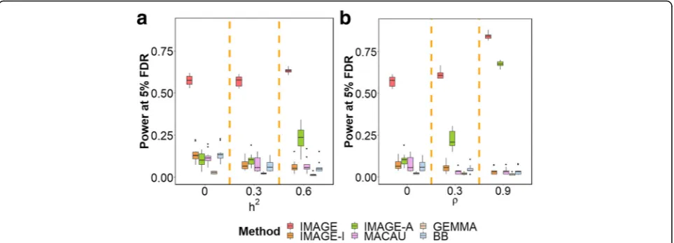
Overall, the simulation results show that IMAGE out-performs all other methods across all tested
parame-ters (Fig. 2 and Additional file 2: Figure S1). For
example, in the baseline simulation scenario, at an FDR of 0.05, IMAGE reaches a power of 57.15% in a sample size of 100 individuals. IMAGE-I, IMAGE-A, MACAU, GEMMA, and BB reach a power of 7.55%, 10.27%, 7.49%, 2.25%, and 6.79%, respectively. The ranking of different methods is not sensitive to differ-ent FDR cutoffs. For example, at an FDR of 0.1, the power of IMAGE is 68.78%, while the power of IMAGE-I, IMAGE-A, MACAU, GEMMA, and BB is 14.98%, 24.35%, 13.64%, 2.84%, and 15.03%, respect-ively. The superior performance of IMAGE suggests that incorporating ASM information into mQTL map-ping can greatly enhance power.
Among the eight parameters we examined, six have similar effects on power across IMAGE and the five
other models we compared. For example, the power
of all methods increases with larger sample size n
(Additional file 2: Figure S1A), larger genetic effect
size PVE (Additional file 2: Figure S1B), larger minor
allele frequencyMAF(Additional file2: Figure S1C), lar-ger read depth TR (Additional file2: Figure S1D), and lar-ger over-dispersion varianceσ2, which implicitly increases the genetic effect sizePVE(Additional file2: Figure S1E). In addition, the power of all methods is the highest for CpG sites with intermediate methylation levelπ0, but re-duced for both hypomethylated and hypermethylated sites (Additional file2: Figure S1F). The power dependence on
π0 is presumably because higher methylation variance in the middle range ofπ0leads to higher power.
Careful examination of the relative performance of dif-ferent methods in difdif-ferent scenarios yields additional
insights. First, among the mQTL mapping methods, we found that count-based approaches (IMAGE-I, MACAU, BB) often outperform a normalized data-based approach (GEMMA). Such performance differences become more apparent when sample size nis small (Additional file 2: Figure S1A), methylation level π0 is either low or high
(Additional file 2: Figure S1F), or mean per-site read
depth TRis low (Additional file 2: Figure S1D). For
ex-ample, when the mean total readTR= 10, the power of
IMAGE-I, MACAU, and BB is 5.8%, 4.56%, and 5.33%,
respectively (n= 100), while the power of GEMMA is
only 1.01%. When TR increases to 30, the power of
IMAGE-I, MACAU, and BB becomes 15.25%, 15.32%, and 14.55%, respectively, while the power of GEMMA remains low, at 6.14%. The superior performance of
count-based methods is consistent with previous
[image:4.595.56.542.89.449.2]observations [40, 57], suggesting that modeling sequen-cing data in the original count form has added benefits for mQTL mapping. For DNA methylation levels, this advantage may arise in part because uncertainty in DNA methylation-level estimates is more accurately modeled in the count data than in normalized ratios. For example, a methylation level of one (completely hypermethylated) is strongly supported for a site-sample combination where read depth is very high, but weakly supported for combina-tions where read depth is low. The count-based methods effectively capture this distinction, which is lost in conver-sion to a single ratio.
Second, ASM-based approaches (IMAGE and IMAGE-A) often outperform mQTL mapping approaches that only use non-allele-specific data. This result holds even for IMAGE-A, even though it only models data for hetero-zygotes at nearby SNPs (and hence, uses only a subset of the data: 42% of the full set of simulated individuals on average). The generally higher power of ASM analysis likely stems from the fact that ASM methods control for
both environmental and trans-acting genetic background
effects (for each heterozygote, both alleles reside in the same individual, providing a natural internal control). Our simulations suggest that there are two important parame-ters that influence the relative power of ASM analysis and mQTL mapping. The first important parameter is back-ground heritability, h2. Increased background heritability can reduce the performance of mQTL mapping methods, as increased confounding from polygenic effects of other SNPs likely increases the difficulty of identifying individual SNP associations [40, 57]. For example, whenh2= 0, the power of IMAGE-I, MACAU, GEMMA, and BB is
13.57%, 11.62%, 2.69%, and 13.88%, respectively. Whenh2 increases to 0.6, however, the power of IMAGE-I, MACAU, GEMMA, and BB reduces to 6.48%, 7.05%, 1.50%, and 5.92%, respectively. In contrast, ASM analysis relies on a model that explicitly accounts for the heritable component that arises from genetic background effects, and thus achieves relatively stable performance. For
ex-ample, whenh2= 0, the power of IMAGE and IMAGE-A
is 57.48% and 10.30%, respectively. Whenh2increases to 0.6, the power of IMAGE and IMAGE-A actually in-creases to 63.07% and 23.09%, respectively. This observa-tion is consistent with the fact that the two alleles modeled in ASM, for each individual, share an identical genetic background that becomes easier to control for as its contribution to DNA methylation increases (i.e., as h2 increases). Thus, IMAGE-I outperforms IMAGE-A when
background heritability is zero (h2= 0), but performs
worse when background heritability is moderate or high (h2= 0.3 or 0.6; Fig.2a).
The second important parameter is the ratio parameter
ρ, which represents the relative contribution of shared/ common environmental effects (i.e., the“trans”acting en-vironment) and also influences the relative power of ASM
vs mQTL. For mQTL methods, increasingρnecessarily
in-creases the contribution of common environmental noise shared between the two alleles. Common environmental noise is not explicitly accounted for by mQTL models, thus leading to a reduction in power. For example, whenρ= 0, IMAGE-I, MACAU, GEMMA, and BB detect 7.55%, 7.49%, 2.25%, and 6.79% of true effects, respectively. When
ρ increases to 0.9, the power of IMAGE-I, MACAU,
GEMMA, and BB reduces to 3.50%, 3.44%, 1.67%, and
Fig. 2IMAGE achieves higher power to detect mQTL across various simulation settings. Power is measured by number of true mQTL detected at a false discovery rate (FDR) of 0.05. Each simulation setting is based on 10 simulation replicates, each including 10,000 simulated SNP-CpG pairs, 10% of which represent true mQTL.aWe varyh2, the background heritability, to be either 0, 0.3, or 0.6, while maintaining other parameters at
baseline.bWe varyρ, the proportion of common environmental variance, to be either 0, 0.3, or 0.9, while maintaining other parameters at baseline. The middle panel inaand the left panel inbcorrespond to the baseline simulation setting. Increasing bothh2andρ, which capture
genetic and common environmental background effects, respectively, results in increased power for methods that use ASM information (IMAGE and IMAGE-A), but losses in power for methods that do not use ASM information (IMAGE-I, MACAU, GEMMA, BB). FDR false discovery rate
[image:5.595.58.540.88.262.2]3.57%, respectively. In contrast, ASM analysis explicitly ac-counts for both common and independent environmental background effects, again because it measures DNA methy-lation in the two alleles in the same individual. ASM methods thus achieve better, not worse, performance with higher values ofρ. For example, when ρ= 0, the power of IMAGE and IMAGE-A is 57.15% and 10.27%, respectively.
When ρ increases to 0.9, the power of IMAGE and
IMAGE-A becomes 84.15% and 67.55%, respectively. Con-sequently, while mQTL methods have similar power as
ASM whenρis small, ASM can outperform mQTL whenρ
is large (Fig.2b).
In addition, we note that IMAGE can estimate FDR rea-sonably accurately by constructing an empirical null via per-mutations. In particular, IMAGE produces either calibrated or slightly conservative FDR estimates regardless of the values ofh2(Additional file2: Figure S2A),ρ(Additional file2: Figure S2B), n (Additional file 2: Figure S2C), genetic
effect size PVE (Additional file 2: Figure S2D), MAF
(Additional file 2: Figure S2E), average read counts
per siteTR(Additional file2: Figure S2F), over-dispersion variance σ2 (Additional file 2: Figure S2G), or average methylation ratioπ0(Additional file2: Figure S2H).
Finally, we note that while we set PVE = 0.10 and h2= 0.30 in the baseline simulations to capture realis-tic effect sizes and background heritability across all SNP-CpG pairs genome-wide, reasonable data filtering
decisions will often increase mean PVE and h2 among
SNP-CpG pairs tested in real data applications. For example, in the wolf and baboon data sets analyzed below, the median PVE was approximately 0.15 and
the median h2 estimate was near 0.5. For direct
com-parability, we therefore also created a simulation
sce-nario in which we set PVE to 0.15 and h2 to 0.50
(Additional file 2: Figure S1G). Notably, the relative
power of different methods in this setting largely re-capitulates our observations in the real data applica-tions (see below).
mQTL mapping in wild baboons
We applied our method to analyze a reduced representa-tion bisulfite sequencing data collected on 67 baboons from the Amboseli ecosystem of Kenya [40, 45]. Detailed data description and processing steps are provided in the “Materials and methods” section, with an illustrative
pro-cessing diagram shown in Additional file 2: Figure S3.
Briefly, we extracted 49,196 SNP-CpG pairs from the bi-sulfite sequencing data, which consists of 13,753 unique SNPs and 45,210 unique CpG sites. We applied IMAGE together with the other five approaches described above to analyze each SNP-CpG pair individually. We performed permutations to estimate FDR for each method, and we report results based on a fixed FDR cutoff.
Consistent with our simulations, our method achieves higher power compared with other methods in the
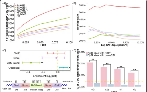
ba-boon data set (Fig. 3a). For example, at an empirical
FDR of 5%, IMAGE detected 7043 associated SNP-CpG pairs, which is 45% more than that detected by the next best method (IMAGE-A, which detected 4855 pairs at a 5% FDR). IMAGE-I, MACAU, GEMMA, and BB de-tected 3585, 3024, 2629 and 3259 pairs, respectively. Also consistent with the simulations, the higher power of IMAGE compared to other methods is robust with re-spect to different FDR cutoffs (Fig. 3a). We illustrate a few example sites that were only detected by IMAGE in Additional file 2: Figure S4. For these sites, methylation levels measured in the heterozygotes are noisy and often indistinguishable from at least one type of homozygote (often because total read counts are unevenly distributed across alleles). However, by separating methylation levels in heterozygotes into the contribution from each indi-vidual allele and modeling ASM information together with non-allele-specific information, IMAGE remains capable of identifying mQTLs in these sites. In addition, consistent with simulations, we also observed that our method could detect more associated SNP-CpG pairs with increasing MAF (Additional file2: Figure S5A), in-creasing read depth TR (Additional file 2: Figure S5B), increasing sample size (Additional file 2: Figure S5C), or
at intermediate methylation levels (Additional file 2:
Figure S5D).
To validate the mQTLs we identified, we randomly split the sample into two approximately equal-sized subsets (one with 34 individuals and the other with 33 individuals) and examined the consistency of the SNP-CpG pairs detected in the two subsets. We removed IMAGE-A from this ana-lysis as it requires at least five heterozygous individuals, which is no longer satisfied for many SNP-CpG pairs in each of the two subsets. For the remaining methods, we found that IMAGE detects more consistent SNP-CpG pairs between the two subsets than the other approaches (Fig.3b). For example, among the top 5% (n= 2511) associated SNP-CpG pairs based on IMAGE, 53.8% of them were identified in both subsets. In contrast, among the top 5% (n= 2511) associated SNP-CpG pairs based on IMAGE-I, MACAU, GEMMA, and BB, 35.84%, 35.12%, 33.92%, and 37.64%
overlapped between the two subsets. The greater
consistency of results from IMAGE thus provides conver-gent support for its increased power.
annotation information from the UCSC Genome
Browser for the baboon genome, Panu2.0, and relied
on the same criterion as [86] to annotate genomic
re-gions (details in the “Materials and methods” section). For each annotated category, we then computed the proportion of mCpG sites in the annotated regions and contrasted it to the proportion of non-mCpG sites analyzed in our original mQTL mapping analysis. We found that mCpG sites are significantly enriched in open seas compared to non-mCpG sites (69.74% vs 66.08%; Fisher’s exact test,pvalue = 0.0106) but
underrep-resented in CpG islands (11.16% vs 14.33%; p value
= 1.056 × 10⁻⁹). The results are consistent with previ-ous observations [87, 88], partly because CpG islands are often enriched in evolutionarily conserved
pro-moter regions [89–91] that harbor fewer regulatory
genetic variants and partly because power to detect
mQTL is lower in hypomethylated regions [92]. The
results are qualitatively consistent across sites with different mean CpG methylation levels, although do not reach statistical significance in all bins likely due to the smaller number of sites and the resulting lower
power in each bin (Additional file 2: Figure S6).
Im-portantly, despite the higher number of mCpG sites detected by IMAGE, the evidence for both enrich-ment in open sea and underrepresentation in CpG islands is also stronger in the IMAGE analysis than for other methods (Additional file 3: Table S1).
Finally, we counted the percentage of SNP-CpG pairs for which the SNP directly resides in the CpG se-quence, abolishing the CpG site and therefore resulting in an entirely unmethylated alternate allele [69, 93].
Fig. 3mQTL mapping results in the baboon RRBS data.aIMAGE identified more mQTL than the other five methods across a range of empirical FDR thresholds.bIMAGE identifies more consistent associations than the other methods in the subset analysis. Here, we randomly split individuals into two approximately equal-sized subsets and analyzed the two subsets separately using each method. We then counted the number of overlapping mQTL identified in both subsets. The overlap ratio (y-axis) is plotted against the percentage of top mQTL ranked by statistical evidence for a SNP-CpG methylation association in each method (x-axis).cUpper panel: log2odds ratio of detecting associated
SNP-CpG pairs, together with the 95% CI, is computed for SNP-CpG sites residing in different annotated genomic regions. SNP-CpG sites with IMAGE-identified mQTL are enriched in open sea regions (pvalue = 0.0106) and depleted in CpG islands (pvalue = 1.056 × 10⁻⁹). Bottom panel: all analyzed CpG sites were annotated to genomic regions based on their relation to the nearest CpG island. CpG islands were annotated based on the UCSC Genome Browser (average length = 672 bp in the data; min = 201 bp; max = 15,960 bp). Shore is the flanking region of CpG islands covering 0– 2000 bp distant from the CpG island. Shelf is the region flanking island shores covering 2000–4000 bp distant from the CpG island.dA higher percentage of CpG sites are directly disrupted by the SNP in mQTL pairs compared to by chance alone (horizontal dashed line), and more so than in non-mQTL pairs (pvalue < 2.2 × 10⁻¹⁶). Such enrichment decays with increased FDR thresholds. *p< 0.05, **p< 0.01
[image:7.595.56.540.89.392.2]These sites, by definition, should exhibit mQTL and ASM. Four hundred three sites in our data set were
dis-rupted by SNPs, and 59.6% of them (n= 240) were
in-deed identified as significant mCpG sites. For 95.70% of
those we did not detect (n= 156), the non-disrupted
CpG was also hypomethylated in our sample (< 10% methylation level), which would make it impossible to detect an mQTL (i.e., because both disrupted and non-disrupted alleles are hypomethylated). CpG sites dis-rupted by SNPs accounted for 3.72% of significant mCpG sites (compared to the 0.89% expected by chance), but only 0.43% of non-mCpG sites, in support of the accuracy of our mQTL mapping approach (Fish-er’s exact testp value < 2.2 × 10⁻¹⁶). In addition, as ex-pected, the percentage of significant mCpG sites accounted for by CpG sites disrupted by SNPs gradually decreases with less stringent FDR cutoffs (Fig. 3d). Im-portantly, IMAGE also outperforms the other five methods on this metric (Additional file3: Table S2).
mQTL analysis in wild wolves
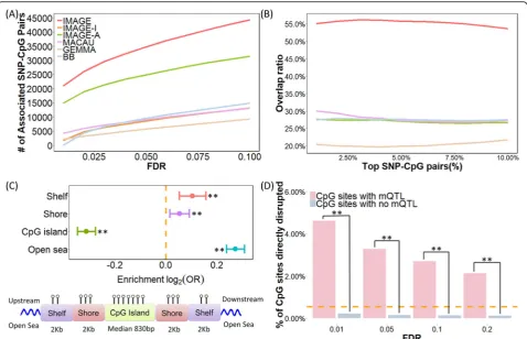
Finally, we applied IMAGE to analyze a second RRBS data set collected on 63 gray wolves from Yellowstone National Park [46,94]. We applied the same data processing proced-ure described above for baboons, followed by mQTL map-ping. In total, we extracted 279,223 SNP-CpG pairs from the bisulfite sequencing data, which consists of 77,039 unique SNPs and 242,784 unique CpG sites. IMAGE again achieved higher power compared with the other methods (Fig.4a). At an empirical FDR of 5%, IMAGE detected 34, 779 significantly associated SNP-CpG pairs, which is 50% more than that detected by the next best method
(IMAGE-A), and 262% more than the other four methods (Fig. 4a
and Additional file2: Figure S7). As in the baboons, subset analysis confirmed that IMAGE detects more consistent SNP-CpG pairs than the other approaches (Fig.4b). For
ex-ample, among the top 5% (n= 14,091) associated SNP-CpG
pairs based on IMAGE analysis, 53.8% of them are consist-ent between the two subsets, compared to 20.5–30.7% for the other four methods tested. Consistent with results from simulations and the baboon data, we also observed that our method could detect more associated SNP-CpG pairs with intermediate methylation levels, increasing MAF, increasing read depth, and increasing sample size (Additional file 2: Figure S5).
Finally, consistent with the baboon results, mCpG sites in the wolves were significantly enriched in open
sea compared to non-mCpG sites (31.77% vs 26.31%;p
value <2.2 × 10⁻¹⁶) and were underrepresented in CpG
islands (30.17% vs 37.43%; p value < 2.2 × 10⁻¹⁶)
(Fig.4c). In the wolves, we also observed significant (al-beit much weaker) enrichment of mCpG sites in shelf regions (12.49% vs 11.63%;p value = 9.001 × 10⁻⁵) and
shore regions (25.57% vs 24.64%; p value = 5.890 ×
10−3). The higher frequency of mCpG sites in CpG
is-land shelves and shores is consistent with previous studies [87,88] and likely reflects greater power to de-tect enrichment in the wolf data set, which yields a lar-ger number of analyzable SNP-CpG pairs than in the
baboons (m= 242,784 in wolf vsm= 45,210 in baboon).
The enrichment in open sea and underrepresentation of mCpG sites in CpG islands are robust regardless of whether we stratify sites based on mean methylation levels, although the shelf/shore results are noisier (Add-itional file 2: Figure S8). Again, we found that enrich-ment results were stronger in the IMAGE analysis than
when using other methods (Additional file 3: Table S3)
and that mCpG sites were more likely to be disrupted by their associated SNPs than non-mCpG sites (3.66% vs 0.18%; p value < 2.2 × 10⁻¹⁶) (Fig.4d; see also Add-itional file3: Table S4).
Discussion
Here, we present IMAGE, a new statistical method with a scalable computational algorithm, for mQTL mapping in bisulfite sequencing studies. IMAGE relies on a bino-mial mixed model to account for the count nature of over-dispersed bisulfite sequencing data, models mul-tiple sources of methylation-level variance, and
incorpo-rates allele-specific methylation patterns from
heterozygous individuals into mQTL mapping. Both simulations and two real data sets support its increased power over other commonly used methods.
A key feature of our method is its ability to incorporate allele-specific methylation information into mQTL map-ping. In RNA sequencing studies, it has been well docu-mented that incorporating ASE information can greatly improve the power of eQTL mapping [51,76–78]. Our re-sults confirm that this observation generalizes to mQTL mapping and provides substantial benefits over approaches that cannot or do not use allele-specific data. Notably, these benefits are not limited to the RRBS data we examined here: IMAGE can also be applied to analyze data generated via whole genome bisulfite sequencing (WGBS) [39] or by newer approaches that distinguish 5-hmc modifications from 5-mc modifications [43, 44]. Doing so would greatly facilitate detection of methylation-associated genetic vari-ants genome-wide, including varivari-ants associated with differ-ent types of methylation marks.
sequencing data [78], or ChIP sequencing data [96], which simultaneously reduces experimental cost and increases the utility of different sequencing data types. Because of these benefits, molecular QTL mapping without separate DNA sequencing or genotyping is gaining popularity [97]. For example, a recent study performed eQTL mapping and ASE analysis using RNA sequencing alone and dem-onstrated that this strategy achieves approximately 50% power compared to traditional eQTL mapping strategies that rely on independently derived genotype data, even though it only uses the 12.66% of SNPs represented in
blood-derived RNA-seq reads [45]. Here, we also show
that genotyping and phenotyping from the same data set can facilitate well-powered mQTL mapping. Notably,
unlike RNA-seq data, because allele-specific methylation information is represented as the ratio between methyl-ated reads and total reads mapped to the same allele, our approach is also less likely to be affected by allele-specific mapping biases (mitigating another argument for generat-ing independent genotype data). Thus, our mQTL map-ping approach has the potential to both increase the utility and applicability of functional genomic data types and improve accessibility of this type of analysis across species.
Our method is not without limitations. For example, to enable ASM-assisted mQTL mapping, our method makes a key modeling assumption that the allelic effect size estimated from heterozygotes is equivalent to the
Fig. 4mQTL mapping results in the wolf RRBS data. Methods for analysis include IMAGE (red), IMAGE-I (orange), IMAGE-A (green), MACAU (pink), GEMMA (brown), and BB (blue).aIMAGE identified more associated SNP-CpG pairs than the other five methods across a range of empirical FDRs constructed by permutation.bIMAGE identifies more consistent associations than the other methods in the subset analysis. Here, we randomly split individuals into two approximately equal-sized subsets and applied methods to analyze the two subsets separately. We count the number of overlapping associations between the top SNP-CpG pairs in the two subsets. The overlap ratio (y-axis) is plotted against the percentage of top SNP-CpG pairs (x-axis).cUpper panel: log2odds ratio of detecting associated SNP-CpG pairs, together with the 95% CI, is computed for CpG sites
residing in different annotated genomic regions. CpG sites associated with SNPs identified by IMAGE are enriched in open sea regions (pvalue < 2.2 × 10⁻¹⁶) and depleted in CpG island regions (pvalue < 2.2 × 10⁻¹⁶). Shores are defined as the 2000-bp regions flanking CpG islands; shelves are
defined as the 2000-bp regions flanking the island shores (2000–4000 bp from CpG islands). Bottom panel: all analyzed CpG sites were annotated to genomic regions based on their relation to the nearest CpG island. CpG islands were annotated based on the UCSC Genome Browser (average length = 830 bp in the data; min = 201 bp; max = 322,257 bp). Shore is the flanking region of CpG islands covering 0–2000 bp distant from the CpG island. Shelf is the region flanking island shores covering 2000–4000 bp distant from the CpG island.dA higher percentage of CpG sites are directly disrupted by the SNP in the mQTL pairs compared to by chance alone (horizontal dashed line), and more so than in non-mQTL pairs (p value < 2.2 × 10⁻¹⁶). Such enrichment decays with increased FDR thresholds. *p< 0.05, **p< 0.01
[image:9.595.59.538.87.395.2]genotype effect size estimated from mQTL mapping across all genotype classes. This assumption is generally satisfied for cisgenetic effects when the SNP is close to
the CpG site [98], and is shared, for gene expression
phenotypes, with ASE-assisted eQTL mapping methods
(e.g., TreCASE and WASP [51, 52]). However, in rare
occasions, the equal effect size assumption may be vio-lated. For example, if ASM arises because of genomic imprinting instead of sequence variation, the allelic ef-fect size may be much smaller than the mQTL efef-fect size obtained across all individuals. Such a violation would lead IMAGE to lose power relative to classical mQTL mapping approaches. Notably, imprinted regions are quite rare in vertebrate genomes (less than 1% of genes are imprinted) [99]. However, excluding imprinted loci prior to IMAGE mapping or substituting the IMAGE-I approach for these loci may slightly improve perform-ance. Additionally, in unphased data, an important limi-tation of IMAGE is that it can only be used to analyze adjacent SNP-CpG pairs that are covered by the same sequencing reads. Analyzing only adjacent SNP-CpG pairs can limit the discovery of mQTLs. Therefore, it would be important to extend IMAGE to analyze distant SNP-CpG pairs in unphased data, using, for example, strategies presented in [100]. Certainly, if SNP data can be phased, IMAGE can also be applied to analyze SNP-CpG pairs that are separated by longer distances. In principle, using phased data could improve mQTL map-ping power even further, if physically linked CpG sites display consistent ASM. Because the baboon and wolf data we analyzed here are not associated with an exten-sive genetic reference panel, we did not attempt to ex-tend our analysis to phased data. Nevertheless, exploring the benefits of phased data or extending IMAGE to ana-lyzing distant SNP-CpG pairs in unphased data is an im-portant future direction.
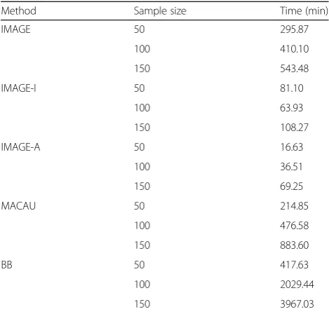
Another limitation of IMAGE is that type I error may not be well controlled when methylation background heritability is high (> 0.6, Additional file 3: Table S5), when the sample size is small (< 100, Additional file 3: Table S6), or when the genotype minor allele frequency is low (< 0.1, Additional file3: Table S7). As a result, we recommend calibrating the false discovery rate against a permutation-derived empirical null, as we have done here (we note that calibrating against permutations has become an increasingly common approach in functional genomic mapping studies in any case [101,102]). Finally, while our method is reasonably efficient and can be readily applied to analyze hundreds of individuals and tens of thousands of SNP-CpG pairs (Table1), new algo-rithms will be needed to adapt IMAGE to data sets that are orders of magnitude larger.
Nevertheless, in its current form, IMAGE is well-suited to analyzing sequencing-based DNA methylation
data sets of the size and scale typically generated in re-cent studies [103]. Thus, it can be flexibly deployed to investigate the genetic architecture of gene regulatory variation, the relative role of genes and the environ-ment in shaping the epigenome, or the mediating role of DNA methylation in linking environmental condi-tions to downstream phenotypes, including human dis-ease (e.g., via Mendelian randomization or related approaches [104,105]).
Materials and methods Method overview
[image:10.595.304.539.142.366.2]Both mQTL mapping and ASM analysis examine one CpG site-SNP pair at a time to identify SNPs associated with DNA methylation levels. However, these two ap-proaches rely on different information to model the genotype-DNA methylation-level relationship. Specifically, mQTL mapping focuses on modeling the methylated read counts and total read counts at the individual level across all samples, without differentiating between the contribu-tions from the two alleles contained within each individ-ual. In contrast, ASM analysis focuses on modeling methylated read counts and total read counts in an allele-specific fashion, restricting it to heterozygotes for the SNP of interest (otherwise, the contributions of each allele can-not be decoupled). mQTL mapping has the benefit of using the entire sample, not just heterozygotes. In con-trast, ASM has the benefit of internal control, since both
Table 1Computational time for analyzing differently sized data sets, for count-based mQTL mapping methods. Computing time is based on analysis of 100,000 SNP-CpG pairs with baseline simulation parameters and varying sample size, using a single thread on a Xeon E5-2683 2.00-GHz processor
Method Sample size Time (min)
IMAGE 50 295.87
100 410.10
150 543.48
IMAGE-I 50 81.10
100 63.93
150 108.27
IMAGE-A 50 16.63
100 36.51
150 69.25
MACAU 50 214.85
100 476.58
150 883.60
BB 50 417.63
100 2029.44
alleles within each heterozygote experience the same gen-etic and environmental background.
To take advantage of both approaches, IMAGE inde-pendently models each CpG-SNP site pair. For each
in-dividual measured at a CpG-SNP pair, we denoteyiand
rias the methylated read count and total read count for the ith individual (combined across alleles), fori= 1,⋯, n. We denote the corresponding methylated and total read counts mapped to each of the two alleles of theith individual as yil and ril, for l= 1 or 2. Thus,yi=yi1+yi2 andri=ri1+ri2. Note thatyilandrilare only observed in heterozygotes, so are treated as missing data in homozy-gotes (more details below). We then model the methyl-ated read counts for each allele as a function of the total read counts for the same allele using a binomial model:
yilBin rð il;πilÞ; ð1Þ
where πil is the true methylation level for the lth allele
in the ith individual. We further model the logit-transformed methylation proportionπil as a function of
allele genotype:
λil¼logitð Þ ¼πil μþxilβþgiþuiþeil; ð2Þ
where μis the intercept;xil is the lth allele type for the
ith individual for the SNP of interest (xil= 0 or 1,
corsponding to the reference allele and alternative allele, re-spectively); and β is the corresponding allele/genotype effect size. In addition to these fixed effects, we model three random effects to account for different sources of over-dispersion. Specifically, gi represents the genetic
background/polygenic effect on DNA methylation for theith individual and can be used to account for kinship or other population structure in the sample. We assume
g¼ ðg1;⋯;gnÞT MVNð0;σ2gKÞ, whereKis a knownn byngenetic relatedness matrix that can be estimated ei-ther from genotype or pedigree data. ui represents
individual-level environmental effects that we assume are independent across individuals but shared between the two alleles within the same individual. We assumeui
Nð0;σ2
uÞ. Finally, eil represents the residual error and
is used to account for independent noise that varies across both individuals and alleles (e.g., stochastic events). We assume eilNð0;σ2eÞ. We standardize the
genetic relatedness matrixKto ensure that the mean of the diagonal elements of Kequals 1, or trðKÞn ¼1. When
this is the case,h2¼ σ
2 g
σ2
gþσ2uþ12σ2e, and can be interpreted as
the approximate background heritability of DNA methy-lation levels (details in Additional file 1: Supplementary Text). Here, the background heritability represents the proportion of variance in the latent parameter λ ex-plained by the genetic effects from all SNPs other than the SNP of focus (i.e., x). Therefore, the background
heritability is the usual heritability minus the genetic ef-fect of x. Our primary goal is to test the null hypothesis that genotype is not associated with methylation levels, or equivalently,H0:β= 0.
While the above model is fully specified for heterozy-gous individuals, it is not fully specified in homozygotes, whereyilandrilare not observed. For homozygotes, only the sums of the reads across both alleles, yi=yi1+yi2 and ri=ri1+ri2, are observed. Therefore, for homozy-gotes, we derive a model foryiandribased on Eq. (1) by summing over all possible values ofyilandril:
P yð ijri;πi1;πi2Þ ¼
X
minðri1;yiÞ
yi1¼0
Xri
ri1¼0
P yð i1jri1;πi1Þ
P yð i−yi1jri−ri1;πi2ÞP rð i1jriÞ: ð3Þ
In Eq. (3), we assume that the model specified in Eq. (1) for the two alleles are independent of each other; thus,P(yi1,yi2|ri1, ri2,πi1, πi2) =P(yi1|ri1,πi1)P(yi−yi1|ri
−ri1,πi2). We further assume that P(ri1|ri) follows a bi-nomial distributionri1~Bin(ri, 0.5), which reflects the as-sumption that both alleles are equally likely to be represented in the sequencing data. Even with these two assumptions, the probability P(yi|ri, πi1, πi2) in Eq. (3) does not have an analytic form and can only be evaluated numerically, which is highly computationally inefficient for parameter estimation and inference. To enable scalable computation, we therefore approximate the distribution in Eq. (3) using a binomial distribution (de-tails in Additional file1: Supplementary Text). Numerical simulations demonstrate the accuracy of this approxima-tion across a range of settings (Addiapproxima-tional file2: Fig. S9).
The model defined in Eqs. (1), (2) (for heterozygous indi-viduals), and (3) (for homozygous individuals) allows us to perform ASM-assisted mQTL mapping to identify SNPs as-sociated with DNA methylation levels. Due to the random effects terms in the model, the joint likelihood based on these equations consists of a high-dimensional integration that cannot be solved analytically. Here, we rely on the pe-nalized quasi-likelihood (PQL) algorithm that is commonly used for fitting generalized linear mixed models [64,80,81] to perform parameter estimation. Based on the parameter estimates, we further calculate a Wald statistic for testing the null hypothesis that H0:β= 0 and obtaining a corre-spondingpvalue.
We refer to the above model as IMAGE, which is im-plemented as a freely available R software package at
www.xzlab.org/software.html.
Simulations
We performed simulations to examine the effectiveness of our method and compare it with other approaches.
To do so, we first randomly selected 150 individuals from the 1958 birth cohort study, which is a part of the control samples that were used in the Wellcome Trust
Case Control Consortium Study (WTCCC) [82]. We
then obtained genotypes for 394,117 SNPs on chromo-some 1 for these selected individuals. In the simulations, we examined the influence of sample size on power by choosing three different sample sizes:n= 50, 100, or 150. For n= 150, we used all 150 samples; for n< 150, we randomly selected the corresponding number of individ-uals from the 150 samples. For each simulation replicate,
we computed the genetic relatedness matrixKfrom the
SNP data using GEMMA [83–85]. We examined the
in-fluence of SNP minor allele frequency (MAF) on power by dividing the 394,117 SNPs into three different MAF bins: an MAF bin centered on 0.1, which contains SNPs
with an MAF between 0.05 and 0.15 (p= 100,631); an
MAF bin centered on 0.3, which contains SNPs with an
MAF between 0.25 and 0.35 (p= 51,800); and an MAF
bin including 0.5 which contains SNPs with an MAF
be-tween 0.45 and 0.50 (p= 23,619). To simulate SNP-CpG
site pairs, given a combination of sample size and MAF bin, we randomly selected one SNP from the appropriate MAF bin and simulated methylation counts and total read counts based on the following procedure.
For the total read counts, we first used a negative
binomial distribution NB(TR,ϕ) to simulate the total
read count ri for each individual. Here, TR is the
mean parameter and ϕ is the dispersion parameter.
We set TR= 10, 20, or 30, close to the median
esti-mate across all CpG sites from the baboon data (de-tails of the data are described in the next section;
median estimate in the real data = 23). We set ϕ= 3,
which is close to the median estimates obtained from the baboon data (median estimate in the real data = 2.80). To obtain the total read count mapped to each of the two alleles, we further simulated a proportion
parameter qi, which represents the proportion of
reads mapped to one allele out of the two alleles. Specifically, qi was simulated from a beta distribution Beta(a,b), where we set the shape parameters a and
b to both be 10, so that the simulatedqi is symmetric
around 0.5 and is within the range of (0.3, 0.7) in 93.6% of cases. With ri and qi, we simulated the total read count mapped to one of the two alleles from ri1~Bin(ri,qi) and set the total read count mapped to the other allele as ri2=ri−ri1.
For the methylated read counts, we performed simula-tions using a combination of five parameters. These five parameters include the intercept μ, which characterizes the baseline methylation level (interpretable as the mean methylation level within a given population); h2, which represents background heritability; σ2, which is the over-dispersion variance;ρ, which characterizes the proportion
of common environmental variance (i.e., for those effects that are shared between the two alleles in each individual) with respect to both the common environmental variance and the independent environmental variance that is independent between both individuals and alleles within
individuals; and PVE, which represents genotype effect
size in terms of proportion of phenotypic variance ex-plained (PVE) by genotype. With these four parameters, we first simulated the genetic random effectsg =(g1,⋯, gn)T(ann-vector) across all individuals from a multivariate
normal distribution with covariance ð1þρÞh2
2þðρ−1Þh2σ2K to guar-antee that the background heritability for our population of simulated individuals is h2 (details in Additional file 1: Supplementary Text). For each individual at a time, we then simulated the environmental random effects (ei1,ei2) andui together as a bivariate vector (ui+ei1,ui+ei2)T from a
bivariate normal distribution with a covarianceΣ, where Σ
¼ ðρð1−pve−h2Þσ2 ρð1−pve−h2Þσ2 1−pve−h2Þσ2 ð1−pve−h2Þσ2
.
For sites where methylation level was not associated
with genotype, the SNP effectβwas set to zero and the
background genetic effects, environmental effects, and an intercept (μ) were then summed together to yield the latent variable πil through logit(πil) =logit(π0) +gi+ui+ eil for the lth allele in ith individual. For sites with true mQTL, we used logit(πil) =logit(π0) +xilβ+gi+ui+eilto yield the latent variable πil, where xil is the allele geno-type for thelth allele in theith individual. We randomly drawβNð0;σ2bÞfor each CpG site in turn, whereσ2bis set to ensure that genetic effects explain a fixed PVE in logit(πil), on average. We setPVEto be 5%, 10%, or 15% to represent different mean mQTL effect sizes, and we derive σ2b ¼ð1−PVEPVEÞσV2ðxÞ, where the function V(•) denotes
the sample variance computed across individuals withx
being a genotype vector of size n. Finally, we simulated the methylated read counts for each allele based on a bi-nomial distribution with a rate parameter determined by the total read counts ri and the methylation proportion
πil; that is,yil~Bin(ril,πil) for the lth allele inith individ-ual. For heterozygotes, we retained the allele-level data (yi1,yi2) and (ri1,ri2). For homozygotes, we collapsed the allele-level data into individual-level data, yi=yi1+yi2 andri=ri1+ri2.
Using the procedure described above, we first
simu-lated data under a baseline simulation scenario of n=
level π0 to be either 0.1, 0.5, or 0.9 to represent low, moderate, or high levels of DNA methylation. We varied
h2= 0.0, 0.3, or 0.6 to represent no, medium, or high
background heritability. We variedσ2= 0.3, 0.5, or 0.7 to represent different levels of over-dispersion. We varied
ρ= 0, 0.3, or 0.9 to represent different levels of common environment influence. For each simulated combination of parameters, we performed 10 simulation replicates consisting of 10,000 CpG sites each. Among these sites, DNA methylation levels at 1000 of them were associated
with the SNP genotype (β≠0) while DNA methylation
levels for the remaining 9000 were not (β= 0).
Baboon RRBS data
We applied our method to a bisulfite sequencing data set from 69 wild baboons from the Amboseli ecosystem
in Kenya [40, 45]. These data were generated using
RRBS on the Illumina HiSeq 2000 platform, with 100-bp single-end sequencing reads. We obtained the raw fastq files from NCBI (accession number PRJNA283632), re-moved adaptor contamination and low-quality bases
using the program Trim Galore (version 0.4.3) [106],
and then mapped reads to the baboon reference genome
(Panu2.0) using BSseeker2 [107] (Additional file 2:
Figure S3; more details in Additional file1: Supplementary Text). After removing two samples that had extremely low sequencing read depths (57,734 and 58,070 reads, respect-ively), sequencing read depth ranged from 5.00 to 79.78 million reads (median = 24.48 million reads; sd = 13.69 million).
We performed SNP calling in the bisulfite sequencing data using CGmaptools, a SNP calling program specific-ally designed for bisulfite sequencing data. CGmaptools examines one individual at a time using the BayesWC SNP calling strategy [78]. Following the authors’ recom-mendations, we used a conservative error rate of 0.01
and a dynamic p value to account for different read
depth per site. Further, we modified the source code to make CGmaptools output homozygous reference geno-types as well. After SNP calling, we indexed and merged variant call files (VCFs) using VCFtools [108]. We then obtained a common set of SNPs where the position was called in at least 50% individuals (including homozygous reference calls). For each individual, we filtered out SNPs that were called using less than three reads. For each SNP, we filtered out variants that had an estimated MAF < 0.05. Finally, we filtered out 989 multiallelic SNPs to obtain a final call set of 289,103 analysis-ready SNPs (mean = 203,864 SNPs typed per sample; median = 204, 554; sd = 34,768). We computed the genetic relatedness
matrixKin GEMMA, using this SNP data set.
To validate the SNP genotype data, we compared the variants identified from the bisulfite sequencing data to a set of previously identified SNP variants in baboons
[109]. These previously identified SNPs were obtained
from 44 different wild baboons from East Africa, includ-ing members of the baboon population from which the RRBS data were generated but also members of baboon populations outside Amboseli, via low-coverage DNA se-quencing (range 0.6× to 4.35×; median = 1.91×; sd = 0.77×). This data set identified a total of 24,770,393 SNPs, with an average of 17,725,780 SNPs genotyped
per individual (median = 18,139,340; sd = 4,315,590).
Because of the low sequencing depth in the DNA se-quencing data set, we expected that variants called from the bisulfite sequencing data would not completely over-lap with variants identified from the DNA sequencing data. Indeed, we found that 50.9% of our called variants are located at a known variant from the DNA sequencing study, with the remaining SNPs being novel. Importantly, among overlapping variants, 99.5% have the same alter-nate allele, in support of the accuracy of SNP calling from bisulfite sequencing data. Additionally, we observe more overlap in called variants with higher alternate allele fre-quency, reaching 72.5% for variants with an alternate allele frequency > 0.5 in the RRBS data (Additional file2: Figure S10A). The allele frequency estimates from the two data sets for overlapping variants are reasonably well correlated (Spearman correlation r= 0.551; p value < 2.2 × 10⁻¹⁶; Additional file2: Figure S10B).
In addition to genotyping, we used CGmaptools to ob-tain CpG-SNP pairs where the SNP and CpG site were profiled on the same sequencing read. The distance be-tween the SNP-CpG site pairs ranges from 1 to 104 bp, with a median distance of 37 bp (mean = 39.75 bp; sd = 26.15 bp; Additional file 2: Figure S10C). We extracted the methylation-level estimates for each CpG site in the form of the number of methylated read counts and the number of total read counts, at the individual level for homozygotes and for each allele separately for heterozy-gotes. We obtained a total of 522,965 SNP-CpG pairs, with 82,217 unique SNPs and 391,137 unique CpG sites. Following [49], we excluded CpG sites (i) that were mea-sured in less than 20 individuals, (ii) where methylation levels fell below 10% or above 90% in at least 90% of measured individuals, (iii) that had a mean read depth less than 5, or (iv) that were paired with a SNP with MAF < 0.05 across individuals for whom DNA methyla-tion estimates were available. To avoid potential map-ping bias, we also excluded CpG sites with apparent differences in methylation levels between reference and alternate alleles that were larger than 0.6. Note that ex-cluding these sites is a conservative strategy and may re-move truly associated SNP-CpG pairs where mQTL are unusually large effect size. After filtering, our final data consisted of 49,196 SNP-CpG pairs, with 13,753 unique SNPs and 45,210 unique CpG sites, and an average of 33,539 SNP-CpG pairs measured per individual.
For these SNP-CpG pairs, the median number of reads per SNP across all individuals was 23 (mean = 31.21; sd = 30.08), and the median number of reads per allele was 13 in heterozygous individuals (mean = 18.75; sd = 19.75). To check the quality of DNA methylation estimates for these CpG sites, we examined their distribution across individ-uals. Similar to other RRBS data sets [110], we observed a bimodal distribution pattern of methylation levels, includ-ing a large number of hypomethylated and hypermethy-lated CpG sites (Additional file 2: Figure S10D). Next, we examined the accuracy of methylation measurements ob-tained from our pipeline by comparing the mean methyla-tion at each CpG site obtained here to those estimated in a previous study that focused on a subset of 61 individuals but used a different mapping and DNA methylation estima-tion pipeline [111]. As expected, the overall distribution of DNA methylation levels is almost identical between our pipeline and the previous study for the 15,605 overlapping sites (Additional file 2: Figure S10E). In addition, site-specific DNA methylation-level estimates are highly corre-lated (Spearman correlationr= 0.855,pvalue <2.2 × 10⁻¹⁶; Additional file2: Figure S10E). Finally, we checked whether our data suggest mapping bias in favor of the reference al-lele. Among the CpG sites we analyzed, we observed no bias in methylation-level estimates between the reference and the alternate alleles (Additional file2: Figure S10F).
We applied five different approaches (details in the “Results” section), together with our primary IMAGE method, to analyze the baboon DNA methylation data. Most of these methods are count based, and algorithms for count-based models can be computationally unstable in the presence of covariates. To control for confound-ing effects from covariates, for each SNP in turn, we removed the effects of age, sex, and the top two
methy-lation principal components based on M values [112]
and used the genotype residuals for analysis. One method, IMAGE-A, requires a relatively large number of heterozygous individuals and was thus only applied to analyze sites for which we identified at least 5 heterozy-gotes (38,250 SNP-CpG pairs). All other methods were applied to all 49,196 SNP-CpG pairs. Because different methods have different type I error control and one method (IMAGE-A) analyzes a different number of SNP-CpG pairs, to ensure fair comparison, we per-formed permutations to construct empirical null distri-butions. Specifically, we combined the count data from the heterozygotes (yi1,yi2), (ri1,ri2) with the count data from the homozygotes (yi,ri), treated the two alleles of each heterozygote as two samples and treated each homozygote as one sample, permuted the sample label 10 times to create null permutations, and applied each method to analyze the permuted data. We note that an alternative permutation strategy would be to permute (yi, ri) along with covariates across individuals. In this
strategy, the number of methylated reads for each allele (out of total reads for each allele) in heterozygotes could then be sampled from a binomial distribution with prob-ability 0.5, conditional on yiand ri−yirespectively. This alternative strategy is not ideal for small sample sizes, but is likely to work well for large samples
(approxi-mately n> 150). Therefore, we have also implemented
this alternative permutation strategy in the software and recommend users to explore both strategies and select one that performs the best for their data. Regardless of which permutation strategy one uses, the statistics from the permuted data allowed us to construct an empirical null distribution. With the empirical null distribution, we estimated the empirical false discovery rate (FDR) for
different methods at different p value thresholds. We
then compared the number of associations detected by different methods at a fixed FDR cutoff.
Finally, following [86], we annotated CpG sites into four categories based on genomic locations obtained from the UCSC Genome Browser: island, shore, shelf, and open sea. CpG islands are defined as short (approxi-mately 1 kb) regions of high CpG density in an otherwise
CpG-sparse genome [113]. A large proportion of CpG
islands have been shown to be associated with gene
pro-moters [114, 115]. The methylation level at the CpG
islands is often associated with transcription repression [116, 117]. CpG shores are defined as the 2 kb of se-quence flanking a CpG island, and CpG shelfs are de-fined as the 2 kb of sequence further flanking CpG shores. Both CpG shores and shelfs have been reported to be more dynamic than the CpG island itself [90, 118,
119]. The methylation variation at shores and shelfs have been associated with various diseases. Finally, the remaining regions outside of CpG island/shore/shelf are
denoted as open seas [120]. We downloaded the CpG
is-land annotations for Panu2.0 directly from the UCSC
Genome Browser, annotated the 2-kb region upstream and downstream of the CpG island boundaries as the shore, annotated the 2-kb regions upstream and down-stream of the CpG shores as the CpG shelves, and anno-tated the remaining regions as open sea (Fig.3e).
Wolf RRBS data
We also applied our method to analyze a second bisul-fite sequencing data set, from 63 gray wolves from Yellowstone National Park in the USA [46,94]. The wolf data are RRBS data collected on the Illumina HiSeq 2500 platform using 100-bp single-end sequencing reads. We obtained bam files for 35 individuals from NCBI
(ac-cession number PRJNA299792) [46] and the fastq files
for the remaining individuals from accession number
PRJNA488382 [94]. We processed all files using the
canFam 3.1 [121] as the reference genome. Per-individual sequencing read depth ranges from 9.53 to 75.18 million reads per individual (median = 31.36 mil-lion reads; sd = 12.91 milmil-lion). We used the same SNP calling procedure described for baboons and applied the same filtering criteria to obtain a final call set of 518,774 SNPs, with an average of 360,063 SNPs genotyped per individual (median = 440,898; sd = 103,522). We also
computed the genetic relatedness matrix K with these
SNPs using GEMMA.
To validate variants identified in the wolf data set, we compared the called variants from the bisulfite sequen-cing data to an existing SNV data base from the current
Ensembl release for the dog genome canFam 3.1. We
found that 17.9% of variants overlapped with known var-iants from Ensembl. Importantly, among overlapping variants, 99.1% of them have the same alternative allele as reported in Ensembl. In addition, the proportion of overlapping variants increases with increasing alternate allele frequency and reaches 41.3% when we focus on variants that have an alternate allele frequency > 0.5 in the RRBS data (Additional file2: Figure S11A).
We followed the same procedure described for ba-boons to extract methylation measurements on CpG pairs. In the wolves, the distance between SNP-CpG site in each pair ranges from 1 to 103 bp, with a median of 35 bp (mean = 38.41 bp; sd = 25.63 bp; Add-itional file 2: Figure S11B). We obtained a total of 861, 474 SNP-CpG pairs, representing 144,670 unique SNPs and 684,681 unique CpG sites. Following quality control filtering, we obtained a final set of 279,223 SNP-CpG pairs, representing 77,039 unique SNPs and 242,784 unique CpG sites, with an average of 179,412 SNP-CpG pairs measured per individual. In this set, the median number of reads per SNP across all individuals is 25 (mean = 31.16; sd = 29.33) and the median number of reads per allele is 14 in heterozygotes (mean = 17.45; sd = 18.90). Methylation levels across sites display the expected bimodal distribution pattern (Additional file2: Figure S11C), and we observed no bias in methylation-level estimates between the reference and the alternate alleles (Additional file2: Figure S11D).
We applied the same analysis procedure to analyze the wolf data as we did for the baboon data set. IMAGE-A was used to analyze 236,092 SNP-CpG pairs where the data set included at least 5 heterozygotes while the other methods were applied to all 279,223 SNP-CpG pairs. We used permutation to construct empirical null distribu-tions for FDR control and controlled for the effects of sex and the top two methylation principal components in the same procedure described in the baboon data. Fi-nally, we annotated CpG sites into island, shore, shelf, and open sea categories as described above, based on the canFam3.1genome.
Supplementary information
The online version of this article (https://doi.org/10.1186/s13059-019-1813-1) contains supplementary material, which is available to authorized users.
Additional file 1:Supplementary text on IMAGE modeling and inference details.
Additional file 2:Supplementary figures on the performance evaluation of IMAGE and on the quality control of the real data applications.
Additional file 3:Supplementary tables on functional enrichment analyses and type I error control examination.
Additional file 4:Review history.
Acknowledgements
We thank Yichen Si at the University of Michigan for helping with the initial exploration of the method. This study also makes use of data generated by the Amboseli Baboon Research Project (ABRP), data generated in the Yellowstone gray wolf population, and the Wellcome Trust Case Control Consortium (WTCCC). A full list of ABRP past and current funding sources and contributors to these data is available athttp://amboselibaboons.nd.edu. A full list of the investigators who contributed to the generation of the WTCCC data is available fromhttp://www.wtccc.org.uk/. Funding for the WTCCC project was provided by the Wellcome Trust under award 076113 and 085475.
Review history
The review history is available as Additional file4. Authors’contributions
JT and XZ conceived the idea and provided funding support. YF and XZ developed the method and designed the experiments. YF implemented the software and performed simulations with assistance from SS and QP. YF and TPV performed real data analysis. YF, JT, and XZ wrote the manuscript with input from all other authors. All authors read and approved the final manuscript.
Funding
This study was supported by the National Institutes of Health (NIH) grants R01HD088558 and R01HG009124 and National Science Foundation (NSF) grants DMS1712933 and BCS1751783. YF is also supported by a scholarship from the China Scholarship Council. Computing in this study is supported in part by the North Carolina Biotechnology Center (Grant 2016-IDG-1013).
Availability of data and materials
Baboon RRBS fastq files are available in the Sequence Read Archive (SRA) of NCBI under accession PRJNA283632 [40,45]. Wolf RRBS bam files for 35 wolves are available under accession PRJNA299792 [46], and the fastq files for the other 27 wolves are available under accession PRJNA488382 [94]. The Trim Galore! Software is available fromhttps://www.bioinformatics.babraham. ac.uk/projects/trim_galore/[106]. The BS Seeker 2 software is available from
http://pellegrini-legacy.mcdb.ucla.edu/bs_seeker2/[107]. The VCFtools software is available fromhttp://vcftools.sourceforge.net/[108]. The CGmaptools software is available fromhttps://cgmaptools.github.io/[78]. The GEMMA [83–85], MACAU [40,57], BB [40], and PQLseq [64] software packages are available fromhttp://www.xzlab.org/software.html.
IMAGE is an open-source R package that is freely available from GitHub [122]
https://github.com/fanyue322/IMAGE, CRAN (https://cran.r-project.org/web/ packages/IMAGE/index.html), andhttp://www.xzlab.org/software.html. Source code for the software release used in the paper has been placed into a DOI-assigning repository [123] (https://doi.org/10.5281/zenodo.3334384). The code to reproduce all the analyses presented in the paper is available on GitHub [124] (https://github.com/fanyue322/IMAGEreproduce) and deposited on Zenodo [125] (https://doi.org/10.5281/zenodo.3334388).
Ethics approval and consent to participate Not applicable.
Consent for publication Not applicable.