Modelling and Temperature Control of Heat Exchanger process

Modelling and Temperature Control of Heat

Exchanger process

Shanu Khan

Deptt. of Elect. Instrumentation & Control, Global Technical Campus, Jaipur

Abstract—The main purpose of a heat exchanger system is to transfer heat from a hot fluid to a cooler fluid, so temperature

control of outlet fluid is of prime importance. In this paper, firstly simplified mathematical model for heat exchanger process

has been developed and used for the dynamic analysis and control design. Artificial neural networks (ANN) are effective in

modeling of non linear multi variables so modeling of heat exchanger process is accomplished using optimized architecture

of artificial neural network after that different controllers such as PID controller, feedback plus feed-forward controller and

a ratio controller are developed to control the outlet temperature of a shell and tube heat exchanger. The main aim of the

proposed controllers is to regulate the temperature of the outgoing fluid to a desired level in the minimum possible time

irrespective of load and process disturbances and nonlinearity. The developed ratio controller has improve the overshoot

from 1.34 to 0 % and settling time from 148 to 91.8 second over the feed-forward plus feedback controller.

Keywords – Artificial neural network, Feed-forward plus feedback controller, Levenberg-Marquardt algorithm, PID

controller, Shell and tube heat exchanger

I. INTRODUCTION

To exchange heat among the two fluids with of the different

temperatures and with higher

efficiency, the heat exchangers are commonly used in the

industries such as gas processing, petrochemical industries

etc. In this work shell and tube heat exchanger is used for

heating or cooling of process fluids. It consists of parallel

tubes enclosed in a shell. Basically they are used for high

pressure applications (with pressures greater than 30 bar and

temperatures greater than 260°C). But the main problem of

heat exchanger process is the temperature deviation from the

desired set point.

Modeling of heat exchanger process for the

estimation of hot and cold fluid outlet temperature as a

function of flow rates and inlet temperature is accomplished

using optimized architecture of artificial neural network. An

neural network 10 to 100 times faster than the usual back

propagation algorithm is the Levenberg-Marquardt algorithm.

While back propagation is a steepest descent algorithm, the

Levenberg-Marquardt algorithm is a variation of Newton's

method. The Levenberg-Marquardt algorithm provides a nice

compromise between the speed of Gauss Newton and the

guaranteed convergence of steepest descent. In this training

algorithm supervised learning has been employed where the

target values for the

output are presented to the network, in order for the network

to update its weights. The various parameters to be taken into

account for developing a model are inlet and outlet

temperatures of shell and tube side fluids and their flow rates.

Artificial neural networks (ANN) are effective in modeling of

non linear multi variables relationship and also referred as the

black box models.

First of all, a classical PID controller is implemented in

a feedback control loop so as to obtain the control objectives.

To further optimize the control performance, feed-forward

controller and ratio controller is used in conjunction with the

PID controller. Auto-tuning of PID controllers is also

implemented and simulated in this paper. A comparative study

of all the control performance is evaluated in this paper.

II. MODELING OF HEAT EXCHANGER

Artificial neural network model is developed using optimized

architecture for modeling of heat exchanger for estimation of

hot and cold fluid outlet temperature as a function of flow

rates and inlet temperature. The data required for these

networks has been generated using water 20% glycerin case.

Following different modes are used to generate data

experimentally.

TABLE I

MODES OF DATA GENERATION Mode Tube side

inlet temperature

Tube side flow rate

Shell side inlet temperature

Shell side flow rate 1 Varied Constant Constant Constant 2 Constant Varied Constant Constant 3 Constant Constant Varied Constant 4 Constant Constant Constant Varied

In this model of actual temperature versus predicted

temperature, the actual heat exchanger data using ‘nftool’ of

MATLAB was used to train the neural network model. The

system automatically takes 60% of data for training, 20% for

validation and 20% for testing, so that the same data will not

be used for testing. It requires many runs to converge or to get

expected training. Once the system was trained then it takes

with remaining samples of data for testing. To identify a first

order plus dead model (FOPDT) parameters two times are

the output reaches 63.2 % of

Y

_F



Y

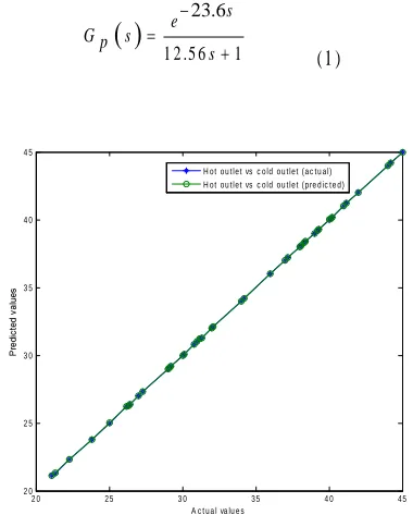
_I. From figure 1,

t

₁ =

27.792 and

t

₂ =36.168. By applying the identification process on the above figure obtained the first order plus dead time

model (FOPDT) as

 

23.6

1 2 .5 6 1 s e

G_p s

s

 

 _{(1 )}

F ig 1 : A c tu a l an d p red ic te d v a lu es o f h o t flu id a n d c o ld flu id

F ig 2 : R e g ress io n p lo ts fo r a c tu a l a n d p red icted res u lts b y fe e d -fo rw a rd n eu ra l n e tw o rk m o d e l fo r tra in in g , v a lid a tio n , tes tin g sa m p le s an d a ll d a ta s et

In fig u re 2 th e d a s h e d lin e is th e p e rfe c t f it lin e w h e re o u tp u ts

a n d ta r g e ts a r e e q u a l to e a c h o th e r. T h e c ir c le s a re th e d a ta

p o in ts a n d c o lo u r e d lin e re p re se n ts th e b e st fit b e tw e e n

o u tp u ts a n d ta r g e ts. H e r e it is im p o r ta n t to n o te th a t c ir c le s

g a th e r a c r o ss th e d a sh e d lin e , s o o u r o u tp u ts a re n o t fa r fro m

ta r g e ts. F r o m th e g ra p h , it c a n b e re a liz e d th a t th e b e st h id d e n

u n it w ith 9 9 % a c c u ra c y is w ith ju st o n e n e u r o n w ith o n e tria l

f o r th is m o d e l.

F ig 3 : S h o w s tra in in g , v a lid a tio n a n d te s tin g m e an s q u a re e rro rs fo r L e v e n b e rg -M a rq u a rd t a lg o rith m w ith o n e n e u ro n .

F ig u r e 3 d e p ic ts th e tra in in g , v a lid a tio n a n d te st m e a n s q u a re

e r ro rs f o r L e v e n b e r g - M a r q u a rd t a lg o rith m w ith o n e h id d e n

n e u r o n s. T h e tra in in g sto p s w h e n M S E d o n o t c h a n g e

sig n ific a n tly .

T A B L E II O P E R A T IN G C O N D IT IO N

P a ra m ete r U n its S h e ll s id e T u b e s id e F lu id - W a te r 2 0 % g ly c e rin T e m p e ratu re

(ra n g e )

c

 3 9 -5 1 1 7 -2 8 F lo w ra te s L P H 5 7 .6 -2 2 5 0 5 7 .6 -2 2 5 0 S p e c ific h e at J /k g K 4 1 8 4 3 4 0 6

V isc o s ity N s /m 0 .7 2×10 1 .4 47 ×10

T h e rm a l c o n d u c tiv ity

W / K 0 .6 6 1 .4 5 5

2 0 2 5 3 0 3 5 4 0 4 5

2 0 2 5 3 0 3 5 4 0 4 5

A c t u a l va lu e s

[image:4.612.75.265.190.432.2] [image:4.612.329.550.262.391.2] [image:4.612.65.279.474.641.2]

TABLE III

PERFORMANCE EVALUATION OF TRAINING, VALIDATION AND TESTING

Number of Hidden Neurons

Operation Samples MSE R 1 Training 27 2.1026e-7 9.99999e-1 1 Validation 9 3.0011e-7 9.99999e-1 1 Testing 9 2.0335e-7 9.99999e-1 2 Training 27 1.5719e-8 9.99999e-1 2 Validation 9 7.8179e-8 9.99999e-1 2 Testing 9 5.6004e-8 9.99999e-1

III. PROBLEM STATEMENT

In this section we have developed a block diagram of these

control loops and modeled the heat exchanger system,

actuator, valve, sensor using the experimental data available.

The transfer function model of the individual systems are

generated which in turn combined to acquire the transfer

function of the whole system.

From the above experimental data the transfer function model

of the system is derived.

Transfer function of process

 

23.6

1 2 .5 6 1

s e G_p s

s  



G a in o f v a lv e 0 .1 3 3

T r a n sf e r fu n c tio n o f v a lv e 0 .1 3 3 3s1

G a in o f I/P c o n v e rte r is 0 .7 5

T r a n sf e r fu n c tio n o f th e r m o c o u p le is 0 .1 6 1 0s1

A . P ID

C o n tr o lle r

T h e c h a ra c te ristic e q u a tio n ( 1 + G (s) * H ( s) = 0 ) in th is c a se is

o b ta in e d a s b e lo w .

3 2

9 0 0s 4 2 0s 4 3s1 .7 8 0

T h e P ID c o n tr o lle r is tra d itio n a ll y su ita b le f o r se c o n d a n d

lo w e r o r d e r s y s te m s. It c a n a ls o b e u s e d f o r h ig h e r o r d e r

p la n ts w ith d o m in a n t se c o n d o r d e r b e h a v io r. A P ID c o n tr o lle r

is tu n e d a c c o r d in g to a ta b le b a se d o n th e p r o c e s s r e s p o n se

te st. A c c o r d in g to Z e ig le r- N ic h o ls f re q u e n c y r e s p o n se tu n in g

c r ite ria

0 .6

K _p  K_c _i  0 .5T 0 .1 2 5T d

 

F o r th e P ID c o n tr o lle r in th e h e a t e x c h a n g e r, th e v a lu e s o f

tu n in g p a r a m e te rs o b ta in e d a r e

0 .2 7 8 1

K p  _i 1 0 .2 _d  2 .55 a n d P  0 .4 6 3 6

0 .0 4 5

I  D  1 .1 8

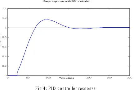
F ig u r e 4 c le a r ly sh o w s th a t th e d e la y w ill a ff e c t th e ste p

r e sp o n s e o f p r o c e ss till th e tim e 2 3 .6 se c . a n d a f te r th a t it

f o llo w th e ste p r e s p o n se .

F ig 4 : P ID c o n tro lle r re s p o n se

N o w d iff e re n t v a lu e s o f i.e . 0 .2 7 8 1 a n d 0 .4 6 3 6 a re u se d Step response w ith PID controller

Time (sec)

[image:5.612.332.548.498.643.2]

[image:6.612.44.301.98.304.2]

Fig 5: Feedback PID controller with different gains

B.

Feedback and Feed-forward Controller

A feed forward control estimates the error and changes the

manipulating variable before the disturbance can affect the

output. To further minimize the overshoot a feed-forward

controller is introduced in the forward path of the process

along with the feedback controller. The combined effect of

feedback and feed-forward controller reduces the overshoot

value.

In feed forward controller we have tried to regulate the flow

disturbance of the input fluid.

G

p

( )

s

is the transfer function

of the process where as

G s

_d

( )

is the transfer function of flow disturbance.

23.6 ( )

12.56 1

e G_p s

s    35 ( ) 25 1 s e G s d _s   

Gain of valve is 0.133

Transfer function of valve 0.133

3s1

Transfer function of thermocouple 0.16

10s1

Gain of I/P converter is 0.75

Figure 5: Feed-forward plus feedback controller response

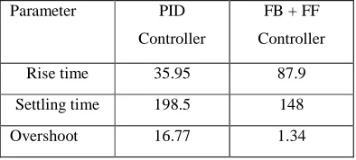
From figure 5, it is clear that feed-forward plus feedback

controller provides much faster response as compared to PID

controller. Also feed-forward plus feedback controller rejects

the disturbance earlier as compared to PID controller.

Overshoot and settling time are less as compared to PID

controller.

A. Comparison of different Parameters in controllers

TABLE III

COMPARISON OF DIFFERENT PARAMETERS IN CONTROLLERS

Parameter PID

Controller

FB + FF

Controller

Rise time 35.95 87.9

Settling time 198.5 148

Overshoot 16.77 1.34

0 100 200 300 400

0 0.2 0.4 0.6 0.8 1 1.2 1.4 From: Tsp

0 100 200 300 400

From: d Closed-loop response to setpoint and disturbance step change

Time (sec)

Feedback only Feedf orw ard + feedback

0 50 100 150 200 250 300 350 400 450 500

0 0.2 0.4 0.6 0.8 1 1.2 1.4 1.6

Step Response of Feedback PID controller with different gain

Time (sec) Amplitude

[image:6.612.340.537.586.675.2]

Peak 1.16 1.01

Peak time 97.10 200

C. CONCLUSION

To efficiently control the temperature, designed three kinds of

controllers and the modeling of heat exchanger is done using

artificial neural network, it can be concluded that the ANN

heat exchanger model using Levenberg marquardt algorithm

for 20% glycerin has been successful and has very good

accuracy level (99% - 99.5%). A classical PID controller is

designed to achieve the control objective. But due to the

unsatisfactory performance of the PID controller a

feed-forward controller is designed and placed in the feed-forward path

of the system. It is observed that feed-forward plus feedback

controller gives a much better response than any other

conventional PID controller.

REFERENCES

[1] Pandharipande S L, Siddiqui M A, Dubay A &

Mandavgane S A, Indian Journal of Chemical Technology,Volume 13, November 2006, pp. 634-639

[2] Mandavgane S A & S L Pandharipande, Indian Journal of Chemical Technology, Volume 13, March 2006, pp 173-176. [3] Mandavgane S A, Siddiqui M A, Dubay A, Pandharipande

S L, Chemical Engineering World, 39(3)(2004)75.

[4] Anderson J A, An Introduction to Neural Networks

(Prentice Hall of India Pvt. Ltd., New Delhi), 1999.

[5] M. Gopal, Control Systems Principles and Design, 2nd ed., New Delhi, India: Tata McGraw- Hill Publishers,2007. [6] G. Stephanopoulos, Chemical process Control, Prentice Hall of India, New Delhi, 1995.

[7] Subhransu Padhee and Yaduvir Singh, “A Comparative

Analysis of Various Control Strategies Implemented on Heat

Exchanger System”: A Case study, “Proceeding of the world congress on Engineering 2010 volume II, WCE 2010, June 30-July2, 2010, London, U.K.

[8] Yuvraj Bhushan Khare and yaduvir singh, “PID control of heat exchanger system”,International Journal of Computer Applications (0975 –8887) Volume 8–No.6, October 2010.

[9] Wolverine tube heat transfer data book.

[10] A Real-Time Approach to Process Control Second

Edition by William Y. Svrcek University of Calgary Calgary,

Canada, Donald P. Mahoney BDMetrics Inc. Baltimore, USA

Brent, R. Young The University of Auckland , New Zealand.

[11] Yang qu, Lin xu, Xiaoke fang, Jianhui wang, and

Shusheng gu, “Neural network predictive control of a heat

exchanger”, International journal of information and systems sciences volume 2, number 1, page 31-41.

[12] Anna vasickaninova, Monika bakosove, Alojz meszaros,

Jiri klemes, “A new approach to heat exchanger control based

on model control”, Chemical engineering transactions volume 21,2010

[13] S.K. Singh “Process Control Concepts, Dynamics and

Applications” PHI Learning Pvt. Ltd. Eastern Economy

Edition, New Delhi 2009.

[14] Donald R. Coughanowr “Process Systems Analysis and Control” McGraw-Hill International Editions,Second Edition, 1991.

[15] I.J. Nagrath, M. Gopal “Control System Engineering”

New Age International (P) Limited,Second edition, August 1997.

[17] B.Sunden and C.A Brebbia “Advanced Computational

Methods and Experiments in HeatTransfer X”, WIT Press

[18] Ramesh K. Shah and Dusan P. Sekulic, Fundamentals of

Heat Exchanger Design, USA:John Willey and Sons, 2003 [19] J.E Normey-Rico and E.F. Camacho, “Control of Dead

Time Processes”, Springer

[20] Jacek M. Zurada, “Introduction to Artificial Neural Systems”, West publishing company

[21] Hagan and Menhaj, 1994: Training feed forward

networks with the Marquardt algorithm. IEEE Trans. on Neural Networks, 5(6), pp.989993.