Detecting Actions of Fruit Flies

(1)

Detecting Actions of Fruit Flies

Eyr´

un Arna Eyj´

olfsd´

ottir

Computing + Mathematical Sciences

California Institute of Technology

A thesis submitted for the degree of

Master of Science

(2)

Acknowledgements

(3)

Abstract

(4)

Introduction

1.1 Motivation

Machine understanding of human behavior is perhaps one of the most useful application of computer vision. It will allow machines to be better aware of their environment, enable rich and natural human-machine interaction, and it will unleash new applications in a number of industries including automotive, entertainment, surveillance and assisted living. Development of automated vision systems that can understand human behavior requires progress in object detection, pose estimation, tracking, action classification and detection, and activity analysis. The focus of this thesis is detection and recognition of actions, which in the case of humans is hampered by two difficulties. First, tracking and pose estimation of humans is very difficult, due to appearance variation, the amount of occlusion in natural environments, and the sheer complexity of human body motions. Second, it is difficult (both technically and legally) to film large numbers of humans behaving spontaneously in natural settings. As a result, human action datasets are small and unrepresentative, especially when social behavior is concerned.

In parallel, neurobiologists are interested in measuring and analyzing behavior of animals of different genotypes, in order to understand the link between genes, brains and behavior. One of their most popular model organism is the fruit fly; it is easy to care for, has a fast life cycle, and exhibits a wide range of behaviors despite having merely 105 neurons. Through a collaboration with biologists we have put together a large annotated dataset of fruit flies interacting spontaneously in controlled environments, which allows us to study natural actions and develop insight into how to represent,

(6)

1.2 State of the art

segment and classify them. If our effort is successful, we can both advance the state of the art in human action analysis and provide biologists with tools for automatic labeling of actions, enabling them to do experiments at a scale which would otherwise be extremely expensive or impossible.

In this thesis we describe an end-to-end approach for detecting the actions of fruit flies from video. The main contributions of our study are:

1. We introduce a new dataset, Caltech Fly-vs-Fly Interactions (Fly-vs-Fly for short), containing 22 hours of continuous video of fruit flies interacting, spontaneously and sporadically. The dataset was annotated by neurobiologists, with complete labeling of 10 social actions. It additionally comes with a second layer of annotations, obtained from trained novice annotators, which can be used as a reference point for action detection performance. Along with the videos, we publish pose (position, orientation, wing angles, etc.) trajectories, from which we have computed a number of time-varying features that may be used to detect, segment and classify actions between the flies.

2. We discuss pitfalls of measures commonly used for benchmarking action detection in continuous video and demonstrate which measures are most suitable, suggesting a protocol for comparing the performance of different algorithms.

3. We define bout features that are designed to extract statistical patterns from an interval of frame-level features and emphasize the similarities of bouts within an action class. Our experiments show that actions cannot be well detected using frame-level features alone, and that bout features improve performance by 28%.

4. We consider two different action detection architectures: sliding window detectors and structured output detectors. By comparing five variants of the two architectures on our dataset, we find that sliding window detectors outperform the structured output detectors, in spite of being orders of magnitude faster.

1.2 State of the art

Datasets: A large number of human action datasets have been published. Most of

the earlier contributions, KTH [1], Weizmann [2], Hollywood 2 [3], Olympic Sports [4], HMDB51 [5], and UCF-101 [6], consist of short pre-segmented action clips, making them

(7)

1.2 State of the art

suitable for action classification, but not for action detection and segmentation. UCF-motion capture [7], HumanEva [8], and CAD-60/120 [9, 10] come with fully tracked skeletons which makes them useful for analyzing a range of human motions; however, these datasets are very small, and their actions are acted. Finally, a recent dataset, VIRAT [11], contains hours of continuous video of humans behaving naturally and intermittently, lending itself well to action detection research; however, the pose of the subjects cannot yet be robustly tracked and the human motion that can be explored is limited; furthermore, VIRAT does not contain social actions. Table 1.1 compares details of the mentioned datasets.

The publicly available datasets of animal behavior videos are Honeybee Dance [12], UCSD mice [13], Home-cage behaviors [14], and CRIM13 [15]. The latter two are suit-able for action detection, containing long videos of spontaneous mouse actions, but both are parameterized with only the tracked centroid of the subject and spatio-temporal features. A large and well annotated dataset containing unsegmented spontaneous ac-tions and including tracking of articulated body motion has not yet been published. Our dataset aims to fill this place.

Dataset Year #Citations Duration* #Actions Natural Social Continuous Articulated

pose

KTH 2004 1397 3 hours 6 x x x x

Weizmann 2005 858 1 hour 10 x x x x

HumanEva 2006 501 22 minutes 6 x x _✓ _✓

UCF-mocap 2007 185 1 hour 5 x x x ✓

Hollywood 2(1) 2009 352(1073) 20 hours 12 _✓ _✓ x x

Olympic Sports 2010 153 2 hours 16 _✓ x x x

HMDB51 2011 83 2 hours 51 _✓ _✓ x x

VIRAT 2011 59 9 hours 12 _✓ x _✓ x

UCF-101(50,11) 2012 16(31,357) 30 hours 101 _✓ x x x

CAD-60/120 2011/13 123/12 2 hours 10** x x _✓ _✓

UCSD mice 2005 1211 2 hours 5 _✓ x x x

Honeybee 2008 51 3 minutes 3 _✓ x _✓ x

Home-cage behs 2010 44 12 hours 8 _✓ x _✓ x

CRIM13 2012 15 37 hours 13 _✓ _✓ _✓ x

Fly-vs-Fly - - 22 hours 11 _✓ _✓ _✓ _✓

* estimated upper limit

[image:7.595.93.507.448.656.2]

** 22 activities, 10 subactivities (actions)

Table 1.1: Summary of existing datasets and our new dataset, shown in chronological order and grouped by human vs. animal. Qualities that are desirable for the purpose of

detecting realistic social actions from articulated pose are highlighted in green.

(8)

1.3 Overview

Action detection: The simplest approach to action detection and classification is frame-by-frame classification, where each frame is classified based a signal on the frame, or on a time window around it, using discriminative or generative classifiers. More sophisticated approaches globally optimize over possible temporal segmentations, out-putting structured sequences of actions. Recent work in action detection falls into these two categories: Dankert et al. detected actions of fruit flies using manually set thresh-olds along with nearest neighbor comparison [16]; Burgos et al. used boosting and auto-context on sliding windows for detecting actions of mouse pairs [15]; and Kabra et al. also use window based boosting for detecting actions of fruit flies in their interactive behavior annotation tool JAABA [17]. Jhuang et al. used an SVMHMM, described in [18], for detecting actions of single housed mice [14]; Hoai et al. used a multi-class SVM with structured inference for segmenting the dance of the honeybee [19]; and Shi et al. used a semi-Markov model for segmenting human actions [20].

We implement variants of the above methods, specifically comparing sliding window SVM detectors against structured output SVM detectors, expecting the latter, which is similar to [14, 19, 20], to improve frame wise consistency and better capture structured actions. For reference, we also compare with the methods described in [17] and [15] and with the performance of trained novice annotators.

1.3 Overview

Figure 1.1 shows the architecture for an end-to-end action detection system, and demon-strates how data flows between user and software. The system takes as input a video of flies, extracts meaningful tracking features for each fly, runs them through an inference algorithm that uses an action model, learnt during a training stage on expert provided annotations, and outputs predicted annotations to the user. The key components in such a system, outlined in Figure 1.1, are: a) collecting a dataset of videos and an-notations that can be used for training and testing a model (Chapter 2), b) tracking flies and extracting meaningful features at each frame (Chapter 3), and c) devising an algorithm for learning an action model, and an inference algorithm that utilizes the model to detect actions from new videos (Chapter 5). Chapter 4 describes performance measures for action detectors, Chapter 6 contains results and analysis of the different approaches, and in Chapter 7 we conclude and discuss future directions.

(9)

1.3 Overview

videos manual

annota tions

Tracking

trajector y

features

Learning

Inference

autom atic

annota tions model

Video acquisition Annotation Data analysis

a)

[image:9.595.95.505.211.484.2]

b) c)

Figure 1.1: System overview: Videos are sent through a tracking module that extracts meaningful features, those features and manual annotations are used by a learning module

to learn an action model, and an inference module uses that model to detect actions from features extracted from new videos. Gray cylenders represent data, blue boxes represent

software, and the cut out section contains components that are used only during training.

The outlined sections represent three major phases of the system: a)Data aquisition, which

involves collecting videos and annotations of actions to be learnt (Chapter 2), b) Feature

extraction, which involves tracking flies in videos and extracting features useful for action

detection (Chapter 3), and c)Training, which involves training an action detection system

from features of annotated actions (Chapter 5).

(10)

2

Fly Data

2.1 Experimental setup

In collaboration with biologists we have collected a new action dataset, Fly-vs-Fly, which contains a total of 22 hours (1.5m frames recorded at 200Hz and 2.2m frames at 30Hz) of 47 pairs of fruit flies interacting. The videos may be organized into three sub datasets according to their preparations:

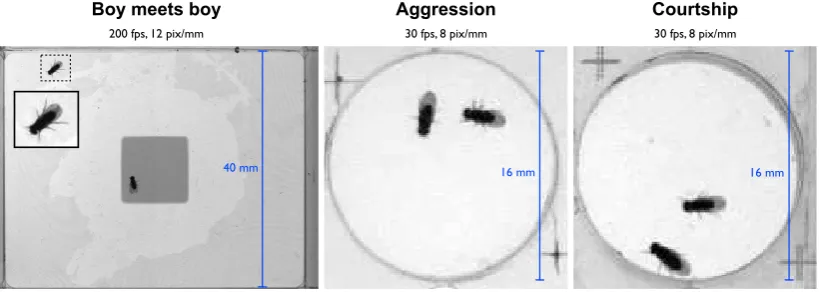
Boy meets boy is designed to study the sequence of actions between two male flies, whose behaviors range from courtship to aggression. The flies are placed in a 4x5 cm2 chamber with food located in the center and walls coated with Fluon such that flies are constrained to walking on the floor. It contains six 20 minute videos recorded at 200Hz with 24 pixels covering the fly body length (2mm).

Aggression contains two hyper aggressive males and is used to quantify the effect of genetic manipulation on their behavior. The flies are placed in a circular 16mm diameter chamber with no food. It consists of ten 30 minute videos recorded at 30Hz with only 16 pixels covering the fly body length.

Courtship has one female and one male fly, which in some of the videos is wild type and in the rest is a so-called hyper courter. This set of videos was used to study how genetic manipulation affects male courtship behavior. It consists of 31 videos recorded with the same chamber and video settings as Aggression, 10 of which contain hyper-courters and the remaining videos with wild type males.

The filming setups for the three different experiments are shown in Figure 2.1.

(11)

2.2 Annotations

16 mm 16 mm

40 mm

Boy meets boy Aggression Courtship

200 fps, 12 pix/mm 30 fps, 8 pix/mm 30 fps, 8 pix/mm

[image:11.595.94.504.143.289.2]

Monday, December 2, 13

Figure 2.1: Experimental setup: Boy meets boyhas high temporal and spatial resolution

videos and a large chamber with food present,Agression andCourtshiphave lower

resolu-tion, a much smaller chamber, and no food. TheCourtshipexperiments contain one male

and one female fly (the larger one), while the other two contain two male flies.

2.2 Annotations

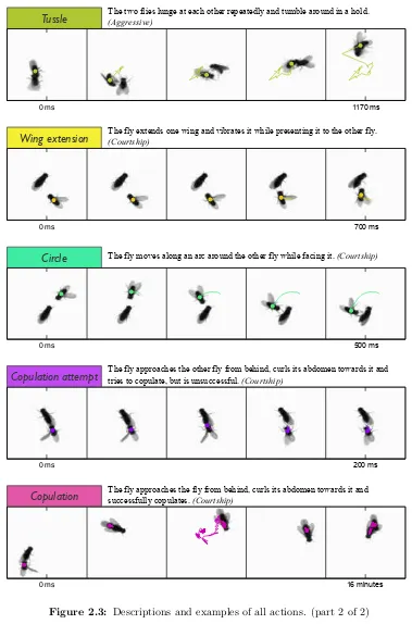
The entire dataset was annotated by biologists, using an annotation tool that comes em-bedded with our tracking tool, with 10 different action classes that they have identified for the study of fruit fly interactions: the introductory behaviortouch, the aggressive behaviorswing threat,charge,lunge,hold, andtussle, and the courtship behaviorswing extension, circle,copulation attempt, and copulation. Figures 2.2 and 2.3 show an ex-ample instance of each of these behaviors, with a sequence of 5 frames subsex-ampled from an action bout, as well as a description of each behavior.

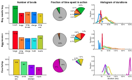
Annotating a video involves finding all intervals within the video that contain an action of interest, also referred to as bouts of actions, and requires recording the start frame, end frame, and class label of each detected bout. The dataset is annotated such that actions can overlap, for instance tussling usually includes lunging, a wing threat sometimes contains charge, wing extension and circling tend to overlap, and touch can overlap with many of the behaviors. The action classes can have substantial intraclass variation both in terms of duration and appearance, and some action instances are am-biguous. Each action takes up only 0.1−7% of the frames, except for copulation which takes up 57% of the Courtship videos. Figure 2.4 summarizes the dataset, showing the number of instances of each action, the fraction of time spent in each action, and a histogram of bout durations for each action.

(12)

2.2 Annotations

Touch

Wing threat

Charge

Lunge

Hold

Tussle

Wing extension

Circle

Copulation attempt

Copulation

The fly touches the leg, wing, or body of the other fly, and in doing so its

gustatory organs sample chemicals that may help identify gender. (Introductory)

The fly extends, and raises, both wings and presents them to the other fly.

(Aggressive)

The fly extends both wings fully and charges towards the other fly. (Aggressive)

The fly raises itself on its hind legs, then slams down onto (or close to) the other

fly’s body. (Aggressive)

After lunging, the fly sometimes holds onto the body of the other fly for an

extended period. (Aggressive)

The two flies lunge at each other repeatedly and tumble around in a hold.

(Aggressive)

The fly extends one wing and vibrates it while presenting it to the other fly.

(Courtship)

The fly moves along an arc around the other fly while facing it. (Courtship)

The fly approaches the other fly from behind, curls its abdomen towards it and

tries to copulate, but is unsuccessful. (Courtship)

The fly approaches the fly from behind, curls its abdomen towards it and

successfully copulates. (Courtship)

0 ms 117 ms

0 ms 70 ms

0 ms 50 ms

0 ms 20 ms

0 ms 96357 ms

0 ms 64 ms

0 ms 230 ms

0 ms 5 ms

0 ms 8 ms

0 ms 250 ms

640 ms

2300 ms

50 ms

80 ms

2500 ms

1170 ms

700 ms

500 ms

200 ms

16 minutes

[image:12.595.106.480.118.697.2]

Wednesday, April 2, 14

Figure 2.2: Descriptions and examples of all actions. (part 1 of 2)

(13)

2.2 Annotations

Touch

Wing threat

Charge

Lunge

Hold

Tussle

Wing extension

Circle

Copulation attempt

Copulation

The fly touches the leg, wing, or body of the other fly, and in doing so its

gustatory organs sample chemicals that may help identify gender. (Introductory)

The fly extends, and raises, both wings and presents them to the other fly.

(Aggressive)

The fly extends both wings fully and charges towards the other fly. (Aggressive)

The fly raises itself on its hind legs, then slams down onto (or close to) the other

fly’s body. (Aggressive)

After lunging, the fly sometimes holds onto the body of the other fly for an

extended period. (Aggressive)

The two flies lunge at each other repeatedly and tumble around in a hold.

(Aggressive)

The fly extends one wing and vibrates it while presenting it to the other fly.

(Courtship)

The fly moves along an arc around the other fly while facing it. (Courtship)

The fly approaches the other fly from behind, curls its abdomen towards it and

tries to copulate, but is unsuccessful. (Courtship)

The fly approaches the fly from behind, curls its abdomen towards it and

successfully copulates. (Courtship)

0 ms 117 ms

0 ms 70 ms

0 ms 50 ms

0 ms 20 ms

0 ms 96357 ms

0 ms 64 ms

0 ms 230 ms

0 ms 5 ms

0 ms 8 ms

0 ms 250 ms

640 ms

2300 ms

50 ms

80 ms

2500 ms

1170 ms

700 ms

500 ms

200 ms

16 minutes

[image:13.595.105.484.139.713.2]

Wednesday, April 2, 14

Figure 2.3: Descriptions and examples of all actions. (part 2 of 2)

(14)

2.2 Annotations

10 10^2 10^3 ₂₃₄₄

95 150 146 77

touch lunge

wing threat

charge _{wing ext.}

92%

6.9% 0.1%

0.9%

0.1% 0.3%

10 10^2 10^3 10^4 10^5 0

0.1 0.2 0.3 0.4

10 10^2 10^3 3195

184 ₁₁₇ ₁₃₂ 410

lunge

wing threat

charge tussle hold

95%

1.2% 2.8%

0.0% 0.2%

0.7%

10 10^2 10^3 10^4 10^5 0

0.2 0.4 0.6 0.8 1

10 10^2 10^3

918 361

83 31

wing ext. circle

coupul. atmpt copulation

57% 41%

1.6% 0.3% 0.1%

10 10^2 10^3 10^4 10^5 0

0.1 0.2 0.3 0.4

duration (ms)

touch lunge wing

threat charge wing ext.

lunge wing

threat charge hold tussle

wing

ext. circle attemptcopul. copul.

B

o

y m

e

ts bo

y

A

g

re

ssion

C

our

tship

Number of bouts Fraction of time spent in action Histogram of durations

fra

ct

io

n

fra

ct

io

n

fra

ct

io

[image:14.595.58.512.138.414.2]

n

Figure 2.4: Action statistics: Left: Number of bouts for each action. Center: Fraction

of time a fly spends in each action, where the gray area represents unlabeled frames and

the right pie shows the unlabeled slices from the left pie expanded exponentially. Right:

Distribution of bout durations for each action class.

In order to get a sense for the difficulty of the dataset, we hired novice annotators and trained them on expert annotations to re-label a subset of the data. Human performance provides a good reference point for evaluating automated action detection but it is not an upper bound; we should strive for performance as least as good as that of humans. Low human performance can result from difference in perception of an action, one annotator may be more or less conservative than another annotator, or some instances of an action may indeed be ambiguous. This, in fact, motivates the use of automated or semi-automated detection systems which enforces consistency between annotations. We discuss the human-human comparison in more detail in Chapter 6, and show that consistency varies substantially depending on the action and whether it is measured at a per frame level or a per bout level.

(15)

3

Data Representation

For action recognition, data representation is half the challenge. If we were to represent a 640x480 pixel resolution video by its grayscale image sequence, then its feature vector would be 307,200 dimensional at each frame, which would require very complex learning algorithms and a large number of training samples. An action classifier should recognize a wing extension, regardless of where within a chamber a fly is standing and which way it is facing, and whether it extends its left or its right wing. In other words, the classifier must be handle any variance within an action class, that does not define the action. To avoid having to work with massive amounts of data and/or requiring extremely complex algorithms, we bring some of our knowledge about the domain into the data representation. When we describe an action we find ourselves saying: it extends its

wings, it raises itsbody, or it touches another fly with itslegs. To capture this we have implemented a system that detects flies, segments them into body parts, and tracks them throughout a video.

raw image segmentation skeleton

[image:15.595.101.499.590.691.2]

Tuesday, December 3, 13

Figure 3.1: Three stages of the tracking process, starting from the raw image of a fly, it’s foreground segmented into body, wing, and legs, and the skeleton fit to those segments.

(16)

3.1 Tracking

We have implemented a tracking tool that extracts fly tracks from raw videos, by de-tecting the flies at each frame, segmenting them into body, wing, and leg components, connecting the detections across frames to form continuous trajectories, and finally pa-rameterizing the body segments to further reduce dimensionality of the representation. A full description of the tool can be found in a separate technical report [manuscript in preparation], but here we describe in short how it works:

Detection: Our system assumes that videos are recorded with a fixed background,

which allows for detection of foreground objects using background subtraction [21]. Given a grayscale video withT frames, {I(t)}_t=1...T, we compute a background image,

Bg, by taking a weighted mean of a subset of equally spaced frames from the video. Us-ing the fact that the flies are dark, we find the foreground at each frame by thresholdUs-ing the background subtracted image. To account for variation in background intensity (for example due to food in the chamber) we normalize the background subtracted image with the background itself, such that the difference on top of darker areas are equally accentuated. The foreground image, F g, at frame t and the foreground mask,f g, are computed as: _{F g} ₌ _|_I₍_t₎₋_Bg_|_./Bg

f g = F g > threshf g

Segmentation: From the foreground mask, we compute masks for the body parts to

be segmented, using the fact that a fly’s body is darker than the remaining part of the fly, its legs are slim, and when body and legs have been removed only wings should remain: _body ₌ _{F g > thresh}_body

legs = f g−dilate(erode(f g))

wings = f g−legs−dilate(body)

Masks are converted to a set of connected components, that are deemed as being a body part of a fly if they satisfy constraints involving the expected size and relative positioning of components, which can be determined form the video resolution. Before assigning wing components, pixels along the major axis of the body ellipse are sub-tracted, such that the wing component gets split into left and right components. In the case when flies are touching, their bodies form a single multi-fly component which we resolve by fitting its mask to a Gaussian mixture model with the appropriate number of components, using an Expectation Maximization algorithm [22].

(17)

3.2 Feature extraction

Individual features

1) velocity 2) angular velocity 3) min wing angle 4) max wing angle 5) mean wing length 6) body axes ratio 7) fg body ratio 8) image contrast

Relative features

9) distance between 10) leg distance 11) angle between 12) facing angle

3)

4) 11)

[image:17.595.95.505.134.271.2]

12)

Figure 3.2:

Illustra-tion of features derived

from the tracked fly

skeletons, which are in-variant of absolute

posi-tion and orientaposi-tion of the fly and relate the

pose of the fly to that of the other fly.

Tracking: Detections between adjacent frames are connected by minimizing the cost of possible assignments. Forndetections in framet−1 andmdetections in framet, we construct ann×mcost matrix where entry (i, j) represents the cost between detection

iin framet−1 and detectionjin framet, measured in terms of the overlap of the body segments and the distance between its centroids. The optimal assignment is found by applying the Hungarian algorithm [23] to the cost matrix.

Parametrization: To narrow down the number of variables even further, we parame-terize the segmented components of the flies. We fit an ellipse to the body components, and represent it as (x, y, a, b, θ), where (x, y) is the centroid of the ellipse, (a, b) are the minor and major axes of the ellipse, andθis its orientation. The orientation of an ellipse has a 180◦ ambiguity, so to determine what is front and what is back we use the following (in that order) for disambiguation: 1) wing position, when wings detected and not extended, 2) heading direction, if velocity is great enough, and 3) consistency with previous frames. Finally, we parameterize the wings by the position of their wing tips (the pixels farthest away from the body centroid), (w_xl, wl_y, w_xr, w_yr).

The tracking tool extracts, for each fly, a sequence of parameters describing its pose: (c, y, a, b, θ, wl_x, wl_y, w_xr, wr_y)t∈{1,...,T}, and to further assist the learning algorithms we

derive a set of features that encode our knowledge about the actions of flies.

3.2 Feature extraction

From the trajectories computed by the tracker we derive a set of features that are designed to be invariant of absolute position and orientation of a fly, and relate the pose of one fly to the pose of the other fly, similar to the approaches of [16, 17]. The features (illustrated in Figure 3.2) can be split into two categories: individual features

(18)

3.2 Feature extraction

which include the fly’svelocity,angular velocity,min and max wing angles,mean wing length, body axis ratio,foreground-body ratio, and image contrast in a window around the fly; and relative features which relate one fly to the other withdistance betweentheir body centers,leg distance (shortest distance from its legs to the foreground of the other fly),angle between, andfacing angle. Analysis of the feature distributions showed that the velocities, wing angles, and foreground-body ratio are better represented by their log values, becoming more normal distributed and better separating actions. Figure 3.3 shows the distribution of each feature, for all actions in the Boy meets boy sub-dataset and the grab-bag actionother, giving an idea of which features are important for which action. For each of the 12 features extracted we additionally take the first two time derivatives, resulting in a feature space of 36 per frame features. We compute these features for each fly, as annotation is done on a per fly basis, which yields double the amount of data for videos containing two flies - more formally, we represent each video by{x1,x2}, wherexi(t) is the vector of per frame features for flyiat frame t.

0.1 1 10 100

0 0.02 0.04 0.06 0.08 0.1 mm/s vel

0.1 1 10 100

0 0.02 0.04 0.06 0.08 0.1 rad/sec ang_vel

0.01 0.1 1

0 0.05 0.1 0.15 0.2 0.25 rad min_wing_ang 0.1 1 0 0.1 0.2 0.3 0.4 rad max_wing_ang

0.6 0.8 1 1.2 1.4

0 0.1 0.2 0.3 0.4 proportion norm mean_wing_length

0.6 0.8 1 1.2

0 0.05 0.1 0.15 0.2 0.25 0.3 proportion norm axis_ratio

2.5 4 6.3 10

0 0.05 0.1 0.15 0.2 ratio fg_body_ratio

0.5 1 1.5

0 0.02 0.04 0.06 0.08 0.1 proportion norm contrast

0 10 20 30

0 0.1 0.2 0.3 0.4 0.5 0.6 mm dist_to_other

0 1 2 3

0 0.01 0.02 0.03 0.04 rad angle_between

0 1 2 3

0 0.05 0.1 0.15 rad facing_angle

0 10 20 30

0 0.2 0.4 0.6 0.8 1 mm leg_dist touch lunge wing threat charge wing extension hold tussle circle copul. attempt copulation frame based bout based

velocity (mm/sec) angular velocity (rad/sec) min wing angle (rad) max wing angle (rad)

foreground/body ratio

normalized mean wing length normalized axes ratio normalized image contrast

facing angle (rad)

distance to other (mm) angle between (rad) leg distance (mm)

log scal e

[image:18.595.87.505.420.702.2]

log scal e fra ct io n fra ct io n fra ct io n

Figure 3.3: Feature distribution shown for the actions of the Boy meets boy sub-dataset,

and for the grab-bag actionother in gray.

(19)

4

Performance Measure

When measuring the performance of an algorithm it is important to use a measure that is relevant to the problem at hand and favors desirable outcomes, which may depend on the objective of the user and the nature of the data (i.e. whether classes are balanced). Here we discuss a few different types of measures and their applicability to the problem of action detection, and describe the difference between a frame based and a bout based measure. For demonstration purposes we have generated synthetic data containing a ground truth sequence with 5 action classes that take up 0.3%−5% of the frames each and less than 8% in total, and two different prediction sequences that are made to emphasize the differences between the various measures.

4.1 Types of measures

A performance measure involves comparison of ground truth labels and predicted labels and can generally be explained in terms of the following (depicted in diagram below): the set of all datapointsS, positivesP, negativesN, predicted positivesP P, predicted negatives P N, true positives T P, false positives F P, true negatives T N, and false negativesF N.

S

P PP

TP

FN FP PN = S/PPN = S/P

(20)

4.1 Types of measures

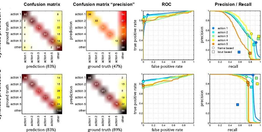
Confusion matrix: Commonly used for multi-class classification, a confusion matrix is a square matrix whose rows contain the normalized distribution of predicted classes for all ground truth instances of a single class, i.e. each entry (i,j) represents the fraction of ground truth instances of class ithat are predicted as class j. An identity matrix represents a perfect result where all instances are correctly classified and a value lower than 1 on the diagonal means that some instances of the class are misclassified, it is therefore common to use the average of the diagonal as a single number to compare the quality of results. This works when classes are balanced within a datasets, but fails when classes are very imbalanced, as is the case with detection problems. In this case the diagonal of a confusion matrix captures well false negatives, but false positives are absorbed into the grab-bag classother which contains a large majority of datapoints. To account for this one must also compare thetranspose confusion matrix, where entry (i,j) represents the fraction of predicted instances of class i that belong to class j according to ground truth. This is demonstrated in figure 4.1 where we show the results for two synthetic prediction examples, both with the same mean on the confusion matrix diagonal but vastly different on the transposed confusion matrix. Effectively, the two matrices representrecall andprecision, which we define below.

ROC:A receiver operating characteristic curve is a common tool to measure quality of detection results for a single class. It plots two values, the true positive rate =T P/P

and the false positive rate = F P/N. A single prediction output can be represented as a single point on the plot, however, most detection algorithms output scores (or probabilities) and all data points whose score is above a threshold are said to belong to the class under detection, so by varying the threshold one can obtain the full ROC curve. This again places little emphasis on false positives; in a dataset with millions of frames, a false positive rate of 1% means there are thousands of false positives, which may be considerably higher than the number of positives. For the purpose of quantifying actions between fruit flies, having more false positives than true positives of a behavior is unacceptable, hence the false positive rate is insufficient to measure the quality of an action detector.

Precision, Recall and F-score: A precision-recall curve is similar to an ROC curve; on one axis it plotsrecall =T P/P, which is the same as the true positive rate, but on the other axis it plotsprecision=T P/P P = 1−F P/P P, which compares the false positives

(21)

4.1 Types of measures 98 2 85 15 95 5 81 19 78 22 99

Transposed mean(diagonal) = 89%

action 1 action 2 action 3 action 4 action 5

other action 1 action 2 action 3 action 4 action 5 other

0 0.2 0.4 0.6 0.8 1

0 0.2 0.4 0.6 0.8

1 Precision / Recall

recall

precision

0 0.2 0.4 0.6 0.8 1 0 0.2 0.4 0.6 0.8 1 ROC

true positive rate

false positive rate

86 14 85 15 72 28 77 23 76 24 100

Confusion matrix −− mean(diagonal) = 83%

other action 1 action 2 action 3 action 4 action 5 other

0 0.2 0.4 0.6 0.8 1 0

0.2 0.4 0.6 0.8

recall precision action 1 action 2 action 3 action 4 action 5 frame based bout based

0 0.2 0.4 0.6 0.8 1

0 0.2 0.4 0.6 0.8

recall

precision

0 0.2 0.4 0.6 0.8 1 0 0.2 0.4 0.6 0.8 1 ROC

true positive rate

false positive rate

36 64 33 67 50 49 53 47 13 87 99 Transposed mean(diagonal) = 47%

other action 1 action 2 action 3 action 4 action 5 other 92 8

2 87 11

4 74 22

4 80 15

2 79 19

9 2 2 86

Confusion matrix −− mean(diagonal) = 83%

other action 1 action 2 action 3 action 4 action 5 other gr ound truth gr ound truth pr ed icti on

ground truth (89%) prediction (83%)

Confusion matrix Confusion matrix “precision”

Synthe tic pr e dic tion 1 Synthe tic pr e dic tion 2

ROC Precision / Recall

true po si tiv e ra te true po si tiv e ra te pr eci si on pr eci si on recall false positive rate

pr

ed

icti

on

ground truth (47%)

[image:21.595.67.514.140.366.2]

prediction (83%) false positive rate recall

Figure 4.1: Results shown for two synthetic predictions compared to a single syntethetic

ground truth. The first two columns show how similar the confusion matrices are for the two examples, but how different their transposed confusion matrices are. The thrid column

shows ROC curves for each class, and the fourth column demonstrates how precision recall curves are able to better reveal the discrepancy between the two examples (points on the

curves represent the 0-threshold). The last column also shows how bout wise and frame wise measurements can differ.

to the total number of predicted positives rather than the negatives. As shown in figure 4.1, this measures emphasizes the difference between the two synthetic predictions better than the ROC curves. For ranking different methods we combine precision and recall into a single value using theF-score, defined as Fβ = (1 +β2)·_β2precision_·_{precision+recall}·recall ,

which forβ = 1 represents the harmonic mean. We prefer the harmonic mean over the standard mean as it favors balanced precision-recall combinations.

We conclude that a confusion matrix is good choice for multi-class detection problems where classes are mutually exclusive, due to its ability to compare classes against each other, but one must also look at the transpose confusion matrix. However, for ex-periments such as ours, where classes may overlap and false positives are expensive, precision-recall curves are the best performance measurement tools.

(22)

4.2 Bout vs. frame

For behavior analysis, correctly counting the number of action instances is equally as important as correctly measuring the duration spent in an action, hence we must also measure performance at a bout level. To do that, we use an overlap criteria that deems a ground truth bout at interval [sg, eg] and predicted bout at [sp, ep] to match only if

min(eg,ep)−max(sg,sp)

max(eg,ep)−min(sg,sp) > threshold.

When multiple bouts fit that criteria, we match only the one with the highest ratio. A predicted output can have high precision-recall when measured on a per frame basis but low when measured on a per bout basis, and vise versa. This can be seen on the precision recall plots in Figure 4.1 and is explained by scenarios listed in Figure 4.2. We define F*-score, a β-weighted mean of F1-frame and F1-bout, as a single metric for comparing different algorithms, where β can be used to control whether emphasis should be placed on bout- or frame-wise performance.

A:

B:

time

time time

time time time

time A:

B:

A:

B:

A:

B: i)

ii)

iii)

[image:22.595.135.446.431.621.2]

iv)

Figure 4.2: Scenarios explaining discrepancies in bout wise and frame wise performance:

i) Under/over segmented bouts →lower bout than frame wise performance

ii) Short missed/false detections →lower bout than frame wise performance

iii) Under/over estimated duration →lower frame than bout wise performance

iv) Offset bout boundaries →lower frame than bout wise performance

(23)

5

Action Detection

In this thesis we focus on action detection by exhaustive classification, in particu-lar we compare two different architectures: Sliding window detection which refers to classifying fixed size windows that move frame-by-frame over a video sequence, and smoothing the predicted labels with post processing, and structured output detection

which refers to detection by optimizing over all possible segmentations of a sequence into actions. Both schemes involve a training algorithm that learns an action classifier from n labeled sequences, {(xi, yi)}i∈{1,...,n}, and an inference algorithm that takes a

new sequencex and predicts y:={yj}={(sj, ej, cj)}, where yj is the jth bout in the segmentation of x, sj and ej mark the start and end of the bout and cj is its class label. We treat the problem of detecting different actions as disjoint detection prob-lems, mainly because the data that we are interested in has many overlapping actions, and because it is more general than a multi-class approach with respect to adding new classes of actions. Before describing the detection architectures in detail we definebout features that aggregate per frame features over an interval of frames, and are used in our implementation of both detection schemes.

5.1 Bout features

We define a number of bout-level features that are designed to extract statistical pat-terns from an interval of per frame features, and emphasize the similarities of bouts within an action class, invariant of their durations. A bout featureψk(x, tstart, tend) is a function of sequencex and interval [tstart tend]; we consider the following:

(24)

5.1 Bout features

Bout statistics featurescapture statistics of frame-features over an interval and can be expressed as: op(x(tstart:tend)), where op ∈ {min, max, mean, std}.

x: time

min, max, mean, std

x: time

min, max, mean, std

x: time

+ - +

x: time

+

-mean

mean

mean mean

mean mean mean

+

-Thursday, December 12, 13

Temporal region featurescapture statistics overr equal subintervals, and are meant to handle the differences within an action composed of r sub actions. They can col-lectively be expressed as: {op(x(tstart+ (i−1)dt : tstart+idt−1))}i∈{1,...,r}, where

dt= (tend−tstart+ 1)/(r−1) and op ∈ {min, max, mean, std}.

x: time

min, max, mean, std

x: time

min, max, mean, std

x: time

+ - +

x: time

+

-mean

mean

mean mean

mean mean mean

+

Harmonic featuresare meant to capture harmonic actions and can be expressed as:

Pr

i=1(−1)imean(x(tstart+(i−1)dt : tstart+idt−1)), where dt= (tend−tstart+1)/(r−1).

x: time

min, max, mean, std

x: time

min, max, mean, std

x: time

+ - +

x: time

+

-mean

mean

mean mean

mean mean mean

+

Boundary difference featuresemphasize the change in features at the start and end of a bout, and help with locating boundaries. They are expressed as:

mean(x(t_start/end : t_start/end+dt)) - mean(x(t_start/end−dt : t_start/end)).

x: time

min, max, mean, std

x: time

min, max, mean, std

x: time

+ - +

x: time

+

-mean

mean

mean mean

mean mean mean

+

Bout change featurescapture the difference in features between the beginning and end of a bout, expressed as: x(tend)−x(tstart).

Global difference featurescompare the mean of a bout to global statistics of data, expressed as: mean(x(tstart :tend))−op(x), where op∈ {min, max, mean}.

Histogram featuresrepresent the normalized distribution of each feature within the bout, expressed as: hist(x(tstart : tend), bins), where bins are extracted from the training data, such that an equal number of frames falls into each bin.

WithK total bout functions applied to each of the N per frame features, the feature representation for a bout ends up being a D = KN dimensional vector, ψ. In our experiments we use two temporal region splits, n ∈ {2,3}, and set the number of histogram bins to be 23, resulting in a total of K = 48 bout features.

(25)

5.2 Sliding window framework

Our sliding window implementation has 4 main components: atraining algorithm that learns a classifier from labeled sequences, a classifier module, an inference algorithm that predicts labels for unseen sequences, and apost processing module that promotes continuity in the prediction labels.

Training: The training algorithm converts each sequence of input labels, {yi} =

{(sj, ej, cj)i}, to indicator vectors, {zi}, that specify whether a frame belongs to an action or not. It extracts normalized bout features over fixed sized windows surround-ing each frame of all sequences, obtainsurround-ing high dimensional data points whose labels are the same as those of the frames around which the windows were placed. With this data it trains a classifier using an iterative scheme that overcomes memory limitations that may be associated with large data, and allows us to indirectly optimize with respect to performance measures that involve the number of predicted positives. At each iteration it learns a classifier from a subset of the data, using a learning algorithm suitable for the classifier type, applies it to all of the data and adds misclassified samples to the training set - repeating until the desired performance measure stops increasing.

Inference: The inference algorithm extracts bout features from a window around each frame inx, normalized with statistics from the training data, and classifies each window using the classifier obtained from the training step. The resulting sequence of scores is thresholded to obtain an action indicator vector, ˆz, whose connected components make up the predicted label sequence, ˆy, assigning each bout the label, start frame, and end frame of its component.

Post processing: Classifying a sequence frame-by-frame often results in noisy labels, that is, within a bout of an action a few frames may be just below a threshold and therefore split the bout into multiple bouts. To account for this we fit an HMM to the scores to achieve smoother transitions: we convert scores to posterior probabilities,

P(x(t)|z(t) = 1) := 1/(1+exp(−score(t))),P(x(t)|z(t) = 0) := 1−P((t)|z(t) = 1), compute priors,P(z(1) =c), and transition matrix,P(z(t+ 1) =ci|z(t) =cj), from the training data, and run the Viterbi algorithm [24] to find the most probable frame-wise sequence of actions. For comparison with previous work [15, 17] we also consider box filtering and Auto-context as a way to smoothen the output.

(26)

5.3 Structured output framework

Classifier: The classifier module consists of a binary classifier and its associated learn-ing algorithm. For comparison with our structured SVM implementation, we choose to use a linear SVM classifier, learnt using the LIBLINEAR implementation described in [25]. The classifier can be substituted by any other binary classifier, such as boosting, regression, neural net, or a generative model.

This approach can be converted to a frame-based detector, by simply substituting the bout features around a frame with its per frame features.

5.3 Structured output framework

Structured output detectors differ from sliding windows in that they optimize over all possible segmentations of a sequence into action intervals, finding the best start and end frame of all bouts, allowing for varying sized intervals.

Structured SVM

We extend the structured SVM [26] to train a model that can be utilized for segmenting sequences into actions, by defining ascore function,f(x, y), which assigns high scores to good segmentations and is used both by the training algorithm and the inference

algorithm, and aloss function,L(y,yˆ), which penalizes wrong segmentations and steers the training algorithm.

Training: The goal is to learn the weights wof a score function from a given training set, such that for each training example the score of the true segmentationyi is higher than the score of any other segmentation y by at least L(yi, y). If these constraints cannot be satisfied, a hinge loss is suffered. To learn these weights we use the primal structured SVM objective:

w∗ ←arg min w kwk

2₊_C1

n

X

i=1

max

y [f(xi, y) +L(yi, y)]−f(xi, yi)

,

which we minimize using a cutting plane algorithm [26] that iteratively finds the most violated constraint: ˆy = arg maxy[f(xi, y) +L(yi, y)]. Searching over all possible seg-mentations is intractable, but since our score- and loss functions are linear in the bouts ofy, dynamic programming [27] can solve for the optimaly.

(27)

Score function: We define a score function f(x, y), which measures how welly seg-ments x into actions and can be represented as the sum of a bout score, unary cost, transition cost, and duration cost, over all bouts in the segmentation:

f(x, y) = X (sj_,ej_,cj₎_∈_y

[wcj ·ψ(x, sj, ej)−τ(cj)−λ(cj−1,(cj))−γ(cj, sj, ej)].

The weightsw_cj are used to calculate the score for a bout of class cj,τ(cj) is the cost

of detecting a bout of class cj,λ(cj−1, cj) is the cost of moving from action cj−1 tocj, and γ(cj, sj, ej) is the cost of spending ej −sj + 1 frames in action cj, which is 0 if the duration is within that action’s standard range (observed in training) and grows exponentially with its distance from the range.

Loss function: The loss function compares a ground truth segmentation y with a

predicted segmentation ˆy and penalizes intervals where the two disagree. It should be constructed such that when the loss is small, then the results from the inference are satisfactory. Since our experiments focus on detecting actions of flies, our objective is to maximize the precision and recall of the actions on a bout-level, while maintaining good per frame accuracy. We define the function as:

L(y,yˆ) = X

(s,e,c)∈y

`c_{f n} e−s+ 1

\

ˆ y,ˆc6=c

(s, e)

+ X

(ˆs,ˆe,ˆc)∈yˆ

`c_{f p}

ˆ

e−ˆs+ 1

\

y,c6=ˆc (ˆs,ˆe)

,

where T

ˆ

y,ˆc6=c(b, e) is the number of frames in ˆy intersecting with [b e] with different action class ˆc6= c,`_{f n}c is the cost for missing a bout of class c, and `ˆc_{f p} is the cost for incorrectly detecting a bout of class ˆc. This loss function softly penalizes predictions where the start or end of the bout is slightly incorrect. On the other hand, since the loss is normalized by the bout duration, it effectively counts the number of incorrectly predicted bouts and, unlike a per-frame loss, long actions are not deemed to be more important than short ones.

Inference: Given a score function, f(x, y), and an input x, the optimal segmentation can be found by solving ˆy = arg maxyf(x, y). Again, similarly to the learning phase, searching over all possible segmentations is intractable but we can solve for y using dynamic programming.

(28)

Semi-structured SVM

This approach is effectively a hybrid of the sliding window SVM and the structured SVM; its inference algorithm optimizes over possible segmentations of a sequence, using dynamic programming, but the classifiers are trained using a linear SVM on fixed bouts from the training set.

Training: We extract bout features from the positive bouts, {(sji_{, e}ji₎_}

i, for each sequencexiin the training set, and from randomly sampled negative bouts. We consider a bout as negative if its intersection with a positive bout is less than half of their union, so that large intervals containing positive bouts and small intervals that are parts of a positive bout are still considered as negatives. Inference involves considering all possible intervals of any duration as potential action bouts, however training on all such possible intervals would be intractable. Instead, we generate a limited number of randomly sampled negatives and use an iterative training process that gradually adds useful negative samples. At each iteration we train a classifier on the current training data, run inference with learnt classifier, and add falsely detected positives to the set of negative training samples - repeating until no new false positives are detected.

Inference: Here the goal is the same as in the structured SVM approach, to find

the optimal segmentation of a new input sequence x, ˆy = arg maxyf(x, y), but with a simpler score function: f(x, y) =P

(sj_,ej_,cj₎_∈_yw_cj ·ψ(x, sj, ej). Again, we solve this

using dynamic programming. We speed up the inference by setting upper limits on the duration of an action, which we obtain from the training set.

(29)

6

Experiments and Analysis

In this chapter we present results for each described method on the Fly-vs-Fly dataset. First, we show how detections of trained human annotators compare to those of experts, to give an idea of the difficulty of each action, then we discuss model selection and compare and analyze the performance of each method, and finally we show how the best method performs on CRIM13 and compare it to published results.

6.1 Human vs. human

We trained novice annotators to learn to detect each action in the Fly-vs-Fly dataset, by showing them a subset of annotated movies, having them annotate another subset and providing them with feedback such that they could adjust their detection criteria. Once trained, they re-annotated a portion of the test dataset, completing all movies for Boy meets boy, 1/10 of movies for Aggression, and 4/15 of Courtship movies, enough to give an idea about the difficulty of each action. Overall, the trained annotators achieved best performance on the Courtship sub-dataset, with bout wise precision-recall over 90% for each action, on Boy meets boy their performance was in the 70−100% range, and on Aggression recall was generally above 80% but precision in the 60−80% range. The annotators described Courtship as being easier to annotate than the other two sub-datasets, with actions seemingly less ambiguous, and the lower precision on Aggression than Boy meets boy can partly be explained by the high commotion between flies as well as lower spatial and temporal video resolution, and partly due to potentially missed detections by the original annotator. Figure 6.1 shows the bout- and frame wise

(30)

6.1 Human vs. human

0 0.2 0.4 0.6 0.8 1 0

0.2 0.4 0.6 0.8

1 Precision / Recall − thresh=0.1

recall

precision

0 0.2 0.4 0.6 0.8 1 0

0.2 0.4 0.6 0.8

recall

precision

0 0.2 0.4 0.6 0.8 1 0

0.2 0.4 0.6 0.8

recall

precision

recall recall recall

pr eci si on pr eci si on pr eci si on

Boy meets boy Aggression Courtship

[image:30.595.90.498.140.280.2]

touch lunge wing threat charge wing extension hold tussle circle copul. attempt copulation frame based bout based

Figure 6.1: Human performance measured in terms of frame based (circles) and bout

based (squares) precision-recall. Note the large discrepancies between bout based and frame based performance for a few of the actions, which is generally caused by over- or

under-segmentation of bouts, or due to the short duration of misclassified bouts.

0 50 100 150 200 250 300 350

−10 −8 −6 −4 −2 0 2 4 6 8 10

0 200 400 600 800 1000 1200 1400 1600 1800

−10 −8 −6 −4 −2 0 2 4 6 8 10

0 200 400 600 800 1000 1200 1400 1600 1800 2000

−10 −8 −6 −4 −2 0 2 4 6 8 10

0 100 200 300 400 500 600 700

−10 −8 −6 −4 −2 0 2 4 6 8 10

0 50 100 150 200 250 300 350

−10 −8 −6 −4 −2 0 2 4 6 8 10

0 200 400 600 800 1000 1200 1400 1600 1800

−10 −8 −6 −4 −2 0 2 4 6 8 10

0 200 400 600 800 1000 1200 1400 1600 1800 2000

−10 −8 −6 −4 −2 0 2 4 6 8 10

0 100 200 300 400 500 600 700

−10 −8 −6 −4 −2 0 2 4 6 8 10

0 50 100 150 200 250 300 350

−10 −8 −6 −4 −2 0 2 4 6 8 10

0 200 400 600 800 1000 1200 1400 1600 1800

−10 −8 −6 −4 −2 0 2 4 6 8 10

0 200 400 600 800 1000 1200 1400 1600 1800 2000

−10 −8 −6 −4 −2 0 2 4 6 8 10

0 100 200 300 400 500 600 700

−10 −8 −6 −4 −2 0 2 4 6 8 10

0 50 100 150 200 250 300 350

−10 −8 −6 −4 −2 0 2 4 6 8 10

0 200 400 600 800 1000 1200 1400 1600 1800

−10 −8 −6 −4 −2 0 2 4 6 8 10

0 200 400 600 800 1000 1200 1400 1600 1800 2000

−10 −8 −6 −4 −2 0 2 4 6 8 10

0 100 200 300 400 500 600 700

−10 −8 −6 −4 −2 0 2 4 6 8 10

Charge (Boy meets boy)

Wing threat (Aggression)

Tussle (Aggression)

Circle (Courtship)

[image:30.595.91.505.363.507.2]

1 sec 1 sec 1 sec 1 sec GT Human GT Human GT Human GT Human

Figure 6.2: Segmentation samples from video sequences, explaining the high bout vs. frame performance discrepancy of selected actions. The upper sequence represents the

ground truth (expert) annotations and the lower shows those of our trained annotators.

precision-recall for each action in the Fly-vs-Fly dataset. Actions that stand out from the average are lunge (BMB) and charge (BMB), with over 90% bout wise performance, charge (BMB) and circle, with much lower frame- than bout wise performance, and tussle and wing threat with lower bout- than frame wise performance. Figure 6.2 shows action segmentation samples that explain this bout- vs. frame wise performance discrepancy. The human performance is a good indicator for what to expect from automatic detection algorithms; we do not expect perfection, due to action ambiguity and imperfections in ground truth annotations, but ideally they should achieve at least as good performance as humans.

(31)

6.2 Method comparison

We compare five action detection methods: frame based SVM, window based SVM, and JAABA backend [17], which all fall under the window based detector framework described in Chapter 5.2, structured SVM (5.3) and semi-structured SVM (5.3).

Model selection: All of the implemented methods have free parameters that affect their outcome, such as the weight of regularization term in the optimization function, the error tolerance for optimization termination, and threshold on output scores. These parameters were set using a parameter sweep on the training dataset, such that optimal bout- and frame wise precision and recall combination was achieved.

In order to account for over-segmentation of the window based SVM, we tested three post-processing methods: Auto-context as described in [15], box-filtering which is pro-posed as a post-processing step for JAABA [28], and HMM fitting. Table 6.1 shows the test performance of each approach, averaged over all actions, and from the results we can infer that: HMM outperforms Auto-context and box-filtering; post-processing im-proves bout wise performance for each method; and bout features significantly improve performance upon per-frame features. For the remainder of this chapter, all results are reported with post-processing applied.

For comparison with JAABA we trained detectors on their bout features, plugging their Boosting implementation into the learning and inference modules of our window based framework. JAABA as presented in [17] does not include post processing, but we include it here for a fair bout wise performance comparison.

Bout wise Bout wise

Bout wise Frame wiseFrame wiseFrame wise

Recall Precision F1-score Recall Precision F1-score F*-score

Window based SVM 0.90 0.46 0.61 0.73 0.74 0.74 0.67

+ Autocontext 0.88 0.50 0.64 0.74 0.76 0.75 0.69 + filtering 0.84 0.63 0.72 0.71 0.74 0.72 0.72

+ HMM 0.85 0.73 0.79 0.76 0.78 0.77 0.78

Frame based SVM 0.80 0.32 0.46 0.55 0.55 0.55 0.50

+ HMM 0.54 0.56 0.55 0.77 0.38 0.51 0.53

JAABA 0.90 0.50 0.65 0.79 0.78 0.79 0.71

+ filtering 0.86 0.67 0.75 0.79 0.78 0.78 0.77

Semi struct SVM Recall Precision F1-score Recall Precision F1-score F*-score

partials negative 0.71 0.81 0.76 0.56 0.87 0.68 0.72 partials not negative 0.69 0.70 0.69 0.43 0.91 0.58 0.63

Structured SVM Recall Precision F1-score Recall Precision F1-score F*-score

Hamming loss 0.81 0.72 0.76 0.75 0.86 0.80 0.78

Bout loss 0.84 0.82 0.83 0.82 0.82 0.82 0.83

Mean performance over all actions

On all d

ata

On lung e and wt

(BMB)

On BMB

Semi struct SVM Recall Precision F1-score Recall Precision F1-score F*-score

regular 0.51 0.79 0.62 0.33 0.97 0.49 0.55

short bootstrap 0.76 0.63 0.69 0.63 0.88 0.74 0.71 two tiered 0.78 1.00 0.88 0.64 1.00 0.78 0.83

On we (BMB)

Table 6.1: Comparison of post-processing schemes for the window based framework.

Results show that post-processing of any kind improves performance for all of the methods, and that bout features significantly improve performance over per-frame features.

(32)

7 2 2 1 1 1

4 3 2 2 3

2 2 3 3 4

4 4 1 3 1

2 2 6 3 1

1 1 1 11

rank

Ranking w emphasis on bout (beta = 0.01)

6 5 4 3 2 1

Frame SVM + HMM

Structured SVM

JAABA + filtering

Semi−struct SVM

Window SVM + HMM

Human

8 3 1 2

3 3 4 3 1

1 2 4 4 2 1

1 5 1 4 2

3 6 3 2

1 1 1 2 9

rank

Ranking w equal emphasis

6 5 4 3 2 1

Frame SVM + HMM

Structured SVM

JAABA + filtering

Semi−struct SVM

Window SVM + HMM

Human

9 2 1 1 1

3 4 5 1 1

1 5 1 4 1 1

5 2 7

2 1 5 4 2

1 1 1 11

rank

Ranking w emphasis on frame (beta = 100)

6 5 4 3 2 1

Frame SVM + HMM

Structured SVM

Semi−struct SVM

Window SVM + HMM

JAABA + filtering

Human

Equal emphasis

[image:32.595.52.503.143.273.2]

Bout emphasis Frame emphasis

Figure 6.3: Histogram of method ranks over all actions, from F*-score computed with varying emphasis (bout-equal-frame). Methods are ordered based on mean rank.

Performance: To measure the performance of our action detectors, we compute preci-sion, recall, and F1-score, on a frame- and bout-wise level, and the F*-score with equal emphasis on bout and frame, which can be used to rank the different methods. Figures 6.9 - 6.11 (at the end of this chapter) show how the different methods compare on each action, showing these measures as well as count- and duration consistency which are representative of what biologists use for quantifying actions in their experiments.

The results show considerable variation in method rank depending on the action, so to get a holistic view we consolidate the results in detector rank histograms, which show the number of times each detector achieved each rank and order methods according to their mean rank. Figure 6.3 shows detector rank histograms for ranking based on F*-scores with varyingβ, emphasizing bout performance, frame performance, and the two equally. Through varying emphases ranking stays consistent, placing the window based SVM at the top (after humans), followed by semi-structured SVM, JAABA, structured SVM, and frame based SVM at the bottom, with the exception being that JAABA moves up to first place when emphasis is placed on frame wise performance.

For a finer resolution view of how the methods line up we show the mean F-scores, averaged over all actions, and the performance as a function of time it takes to run the detector on 1 million frames, in Figure 6.4. This view preserves the rank observed in Figure 6.3, but it also shows that most methods cluster around the 70% performance, apart from humans at around 85% and frame based SVM at around 50%. In addition, it shows that the window based methods, performing slightly better than the structured output counterparts, are orders of magnitude faster.

(33)

−1 −0.5 0 0.5

−0.5 0 0.5

PC 1

PC 2

bout emphasis

Human Frame SVM + HMM Window SVM + HMM Semi−struct SVM Structured SVM JAABA + filtering

−0.5 0 0.5

−0.6

−0.4

−0.2 0 0.2 0.4 0.6

PC 1

PC 2

−1 −0.5 0 0.5

−0.5 0 0.5

PC 1

PC 2

equal emphasis

−0.5 0 0.5

−0.4

−0.2 0 0.2

PC 1

PC 2

−1 −0.5 0 0.5

−0.4

−0.2 0 0.2 0.4

PC 1

PC 2

frame emphasis

−0.5 0 0.5

−0.4

−0.2 0 0.2

PC 1

PC 2

0 0.2 0.4 0.6 0.8 1

F1−bout

F1

−

frame

Mean F−score performance

10^0 10^1 10^2 10^3 10^4

0.5 0.6 0.7 0.8 0.9

Inference time for 1m frames (minutes)

Mean F*

−

score

Performance vs time

Mean F1-score Performance vs. time

[image:33.595.142.449.132.283.2]

real &me (30 Hz)

Figure 6.4: Left: Comparison of F1 scores of each method, averaged over all actions. Right: F*-score of each method as a function of approximate inference time.

Analysis: The summary measures described above abstract away information about

performance patterns that may exist between methods and actions. To explore that, we cluster methods based on their F*-score on each action, by first applying principal component analysis to the #methods×#actionsF*-matrix, eliminating correlations, and then applying k-means to the dimension-reduced matrix, splitting methods into 4 groups. Similarly to the detector rank histograms we perform this analysis with emphasis on bout, frame, or equal emphasis, to see whether clusters remain consistent (see Figure 6.5). With equal- and frame wise emphasis, the window based SVM and JAABA form a group, the structured output methods form another one, and humans and frame based SVM are singletons. With emphasis on bout performance, the window based SVM, semi-structured SVM and humans form one group while the remaining methods are singletons. A perhaps more interesting grouping is the converse, where we cluster actions into 4 clusters based on the transposed F*-matrix. A group that is consistent across emphases contains lunge, charge, and copulation attempt, which all share the characteristic of being short and concise but poorly captured by the frame based detector. Wing threat and tussle are also consistently grouped together, both sharing the property of high appearance- and duration variation. Wing extension and touch are almost consistently grouped together, they can both be somewhat defined by a feature (wing angle, leg distance) exceeding a threshold for an extended period of time, and on both actions the frame based detector performs competitively. The final notable observation is that copulation is a singleton in the bout wise grouping, being the only action with near-perfect performance by all methods.