Performance Evaluation of Convolutional Encoders with Different Constraint Rates

Performance Evaluation of Convolutional Encoders

with Different Constraint Rates

Ekwe, A. O1, Iroegbu, C2, Okoro, K. C3

1

Department of Electrical/Electronics Engineering, Mouau, Abia, Nigeria

2

Department of Electrical/Electronics Engineering, Mouau, Abia, Nigeria

3

Department of Electrical/Electronics Engineering, Mouau, Abia, Nigeria

Abstract- This paper is on the performance evaluation of convolutional encoders of different rates with consraint length 7 and

viterbi decoders. Shannon’s capacity theory has shown that it is theoretically possible to transmit information over a channel at any rate with an arbitrary small error probability. Path loss and path fading can introduce errors to the signal during propagation, thus channel coding is introduced to overcome these problems. Convolutional codes are non blocking codes that can be designed to either correct or detect errors. The approach adopted in this research was to use information from various technical journals, research data and world-wide user’s experiences to evaluate configurable rate convolutional encoder with Viterbi decoder from a mother code rate 1/2 and a constraint length 7 with other higher rates of 2/3, 3/4 and 5/6 to ascertain their performances. The Convolutional encoders have proved to be a veritable tool for reducing the effects of noisy transmission channels.

Key Words: Convolution, Encoding, Viterbi, Decoding, Evaluation

I. INTRODUCTION

Shannon’s seminal papers of 1948 and 1949 demonstrated that

by proper encoding of the information, error induced by a noisy channel could be reduced to any desired level without sacrificing the rate of the information transmission [1]. Certain of the reasons for the increasing applications of coding are external; the anticipated rapid growth in space and satellite communications, the revolution in digital integrated circuits, the increasing emphasis on the reliable transmission of digital data and of digitally coded analog signals, the availability of inexpensive computers for systems algorithm and hardware simulation, the increasing digitalization of modems, switches and interconnect facilities, permitting ready interfacing and common maintainability, and the increasing sophistication of the user community[2]. Convolutional encoders with Viterbi decoders are techniques used in correcting errors which are

making it suitable to be transmitted over the communication channel which can either be a wired or wireless system. One function of a modulator is BPSK which is used for modulating high carrier frequency codeword. On entering the channel which is a physical medium used for information transmission, the waveform is affected by noise existing in the channel which could be in form of thermal, crosstalk and switch impulse. This waveform is then reduced to a sequence of numbers by the demodulator in which the acquired channel errors are processed and an error free output sequence produced which matches the estimated transmitted data symbols and termed the received sequence. The channel encoder tries to reproduce the main signal sequence by using the knowledge of code employed by the channel encoder and the redundancy present in the received signal. The source decoder receives the output information from the channel encoder and translates this sequence of binary digits into an estimate of the output source which it then forwards to the information sink. Information sink stand as the final destination to the main signal that was transmitted.

From our explanation, one can infer that these whole operation processes as described above are carried out in a forward and reverse order at the sending and receiver end respectively so as to recover back the initial transmitted signal [4].

II. CHANNEL CODING

Channel coding for error detection and correction helps the communication system designers to reduce the effects of a noisy transmission channel. Error control coding theory has been the subject of intense study since the 1940s and now being widely used in communication systems. As illustrated by Shannon in his paper published in 1948 [5], for each physical channel there is a parametric quantity called the channel capacity C that is a function of the channel input output characteristics. Shannon showed that there exist error control codes such that arbitrary small error probability of the data to be transmitted over the channel can be achieved as long as the data transmission rate is less than the capacity of the channel.

During digital data transmission and storage operations, performance criterion is commonly determined by BER. Noise in transmission medium disturbs the signal and causes data corruptions. Relation between signal and noise is described with SNR (signal-to-noise ratio). Generally, SNR is explained with signal power / noise power and is inversely proportional with

BER. It means, the less the BER result is the higher the SNR and the better communication quality [6].

A Convolutional Codes

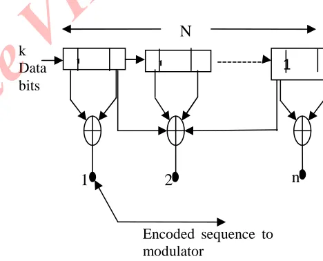
Convolutional codes are linear codes over the field of one-sided infinite sequences. Its usage is regularly seen in the correction of errors existing in a badly impaired channel due to their high affinity to error correction. These codes are recently majorly used in place of block codes when FEC is needed and have been registered to perform exceptionally well when run with Viterbi decoder which can be in the form of soft decision decoding or probabilistic decoding algorithm [7]. The major difference between convolutional codes and block codes is that in block codes, the data sequence is first mapped out into individual blocks before it is encoded, whereas in convolutional codes, there is a direct mapping of that continuous information bit sequence to an encoder output bit. Figure1 below represents a generalized block diagram of a convolutional encoder. According to Rappaport and Theoddore [7], with reference to Figure 1, convolutional codes are generated by simply transmitting the data sequence across a finite shift register with

‘N’ k-bits stages and a linear algebraic function generator ‘m’.

A shift of data ‘k’ bits at any particular time in the shift register

is recorded for every input of the data into the shift register and

an output bit of ‘n’ bits is got for each ‘k’ bit user input.

Fig-1: A generalized block diagram of Convolution encoder

The rate of an encoder is said to be ½ if the encoder outputs two bits for every one bit input. Therefore an encoder with ‘k’ input bits and‘n’ output is said to possess a rate of ‘k/n’ which is

k Data bits

1 --- 1 --- --- 1

1 2 n

N

simply defined as the code rate (Rc) of the system. Figure 2

below is a typical ½ rate binary linear convolutional encoder

with constraint length7.

Fig-2: A convolutional Encoder of Rate 1/2, Constraint length 7

B. Viterbi Decoding

This was first revealed in an IEEE transaction in 1967 [9] having been developed by Andrew J. Viterbi. It makes use of the Viterbi algorithm in decoding a bit stream which has been encoded with a convolutional code. It estimates actual bit sequence using trellis diagram. The decoder examines an entire received of a given length and computes a metric for each path and makes a decision based on this metric. All paths are followed until two paths converge on one node. Then the path with a higher metrics is kept, and the one with a lower metric is discarded. The paths selected are called the survivor. As it can be seen in Figure 3 below, our proposed block diagram of Viterbi decoder is made up of two major working blocks which are the Add and Compare Select (ACS) module and the Path Memory (PM) module with the former handling the BranchMetric calculations, Path Metric calculations and Add-Compare-Select, the latter keeps record and outputs the decoded information bits of the surviving path [10].

Fig-3: Viterbi decoder architecture for a convolutional code of

rate ½ and constraint length.

1 Branch Metric Calculation

Under this part of Viterbi algorithm, an assumption in its design has it that only two paths can lead to any other state of convolutional encoder. This is seen as a calculation of the difference in the input pair of bits and the other four obtainable

ideal pairs which are; ‘00’, ‘01’, ‘10’, ‘11’.

2. Path Metric Calculation

Under this part, a calculation of a metric is made for the pathway, with the least metric (survivor path) terminating in this

state for every encoder. It computes the metrics for ‘2L-1_{’ path,}

choosing one of the paths as the optimal and stores the decisions result in the back tracing unit.

3 Back Tracing

This takes care of hardware implementation with minimal storage of information with respect to the pathway exhibiting a minimum metric path. It stores just a bit decision each time a minimum metric path is selected between the two. The traceback unit uses a convers direction to reinstate the maximum probability path from the result handed in by the path metric unit, making the Viterbi decoder to employ a traceback pattern of First-In-Last-Out (FILO) to recover the data. Figure4 below exhibits these above three discussed different parts of Viterbi algorithm.

Fig-4: Viterbi Decoder Data Flow

C. Parameters that affect the system performance

1Constraint Length

This is said to be the number of bits contained in the encoder memory which influences the number of output bits being generated. Results of experiments carried out has proved that as the constraint length increases, the Bit Error Rate decreases First Output

Second Output

Z-1 Z-1

Z-1 Z

-1 1 1 1 1 1 0 0 1 1 1 BM 0 Path Mem ory ACS BM 1 BM 63 ACS 63 ACS Input Output

ACS MODEL _{PM MODEL}

while the time required to decode and reconstruct the original information also increases. Therefore, we can say that the decoding complexity of a system increases exponentially with the increase in constraint length.

2 Code Rate

This is defined as the measure of the efficiency of the code. Results of previous works carried out on the convolutional coding of different code rates have proved that the transmitting bandwidth employed for equal data transmission in each different code rate decreases with the increase of the code rates. As code rates increases, the Bit Error Rate for the same Signal-to-Noise Ratio decreases. This brings us to the fact that high code rate requires a much lower transmitting power than their preceding lower rates. The efficiency of code rate increases with the increase in the code rates, therefore a code rate of 5/6 will have a higher efficiency than a code rate of 1/2.

3 Soft and Hard Decision Decoding

These are the quantization types implemented on the received bits. Hard decision employs the use of 1-bit quantization

precision of values less or equal to ‘zero’ to be assigned a ‘one’ and values greater than ‘zero’ to be assigned a ‘zero’ on all the

values received on the channel. On the other hand, soft decision uses a multi-bit quantization precision on the same received channel values in its implementation. Therefore we can say that

soft decision decoding requires a stream of ‘soft-bits’ where there is a clearer indication of certainty in the correctness or our

decision and not just were we consider only a ‘one’ or a ‘zero’

to each of our received bits as done in hard decision. When hard decision decoding is implemented, VA computes the hamming distance and its operation is based on discovering a path which possesses the least hamming distance with respect to the received sequence. Therefore we can say that in decoding convolutional codes using hard decision, our target will be to select a path across the trellis with a codeword, C and having a least hamming distance from the quantized received sequence. Soft decision technique is more reliable to give a better decoding result compared to hard decision technique as it has the ability to detect errors even in sequential bits exhibiting both low confidence for error bits and high confidence for non-corrupted bits.

In conclusion, we can say that soft decision decoding is more suitable for AWGN channel as it is preferred to hard decision

decoding because it can correctly decode whatever corrupted sequence with one or two errors irrespective of the level of quantization assigned to the received sequence symbols, whereas hard decision decoding can only detect number of errors less or equal to the code correction capacity.

4 Puncture Pattern

Puncturing generally is a tool universally employed to increase the code rate of convolutional encoder with its matrix applied to the output sequence in a cyclic manner. It is got by eliminating some of the input bits of normal codes implying that not all the bits will be transmitted to the channel. One of its advantages is that the resultant code possesses a high data rate although with a

less error correcting probability. It exhibits ‘ones’ and ‘zeros’ as its matrixes elements with ‘ones’ indicating a bit transmission and ‘zero’ a bit drop. Its operation works in such a way that as

the code rate is being increased, the free distance ‘dfree’ is being

decreased at the same time. These activities bring about a worst case in error performance rate in comparison to when the codes are not punctured.

2.3.5 Polynomials

This is what gives the code its outstanding quality for error protection. With respect to the polynomial chosen, a code can display a totally different behavioral property from the other and since a lot of choices exist for any number of memory register code order, the probability that all will give a good error protective properties for all output sequence is not guaranteed. A polynomial function explains the links that exists among the cell registers which build up the output stream. Our generator polynomial for this work is [171, 133] octal.

III. METHODOLOGY

Fig-5: A communication system model block diagram exhibiting the Convolutional Encoder and Viterbi Decoder

Specifications for Modeling

1. A binary convolutional encoder of rate 1/2 code, 6 memory storage units, constraint length K of 7, 2/3, 3/4 and 5/6 configurable rates with generator polynomial of [171, 133] octal.

2. A soft input Viterbi decoder to take care of the convolutional

encoder in ‘I’.

3. BPSK modulation technique.

4. A binary random data generator as information production unit which should be able to hand in at least 5 million bits of information so as to account for a useful BER data.

5. An SNR bit Eb/Noof 0dB to 10dB.

IV. RESULTS ANALYSIAND DISCUSSIONS

In Figure 6 below, convolutional encoder data simulation was carried out on an input sequence of 1 million bits ranging from 0

to 10dB SNR values and 0.5 line spacing in other to obtain a good performance curve. As can be seen from the graph label, the curve of the convolutional encoder of rate 1/2 and K=7, with Viterbi decoder using hard decision decoding of two-level

quantization signals which is converted to only ‘ones’ and ‘zeros’ over an AWGN channel is marked with blue in the graph

below, and subsequently, curves of 2-bits, 3-bits and 4-bits soft decision decoding are presented in the same Figure for

comparison. The reference curve being the theoretical BER ‘un

-coded’ is also present for use in the verification, comparison and

analysis of the differences in the coding gain of the individual curves. From the hard decision decoding curve, the coding gain

in SNR at a BER of 10-5rated about 3.2dB presenting a decrease

in the amount of transmit power up to a factor of 2 in comparison with the theoretical signal. We also observed that when soft decision decoding was implemented, which involved

the quantization of signals into levels order than just ‘zeros’ and

‘ones’, the gain received increased which means that there was

an improvement in the reduction of transmit power required. When 2-bit soft decision decoding which involves 4-levels (00, 01, 10, and 11) of quantization was implemented, an additional

gain of 1dB SNR at a BER of 10-5 was got in comparison to

when hard decision decoding was used. This also improved to 2.1dB when 3-bit soft decision decoding was implemented and compared with that of hard decision decoding. On increasing to a 4-bit soft decision decoding, little or no significant change was recorded when compared with its 3-bit counterpart.

Fig-6: BER vs SNR curve of different quantization widths for rate 1/2 Binary

BER Random

Binary Generator

Convolutional Encoder

BPSK

Modulator AWGN

Channe l

Tx Error Rate Rx Calculation

BER vs SNR Plot

Soft Output BPSK Demodulator Quantizer

Out1 In1 Viterbi

Decoder

0 1 2 3 4 5 6 7 8 9 10

10-6 10-5

10-4 10-3 10-2 10-1 100

Eb/No in dB

Using configurable rate of 2/3 as shown in figure7, it is observed that BER for each quantization width decreased exponentially with the increase in SNR. The coding gain of each

of them at 10-5BER showed some slight differences with the

4-bit quantization having the best gain of 4.28dB. On the other hand, the percentage rate of bandwidth usage was seen to increase with the decrease in coding rate.

Fig-7: BER performance of rate 2/3 convolutional encoder.

Using configurable rate of 3/4 as shown in figure 8 below, the coding gain when measured showed that the 2-bit quantization

width exhibited a coding gain of 3.4dB at a BER of 10-5, 3-bit

quantization width showed a 4.0dB value at the same BER of

10-5, while the 4-bit quantization gave the same value as that of

the 3-bit quantization. This indicates that an increase in the quantization bit after the third bit does not really have a significant effect or much better BER performance but rather takes a longer computational time to simulate and produce results.

Fig-8: BER performance of rate 3/4 convolutional encoder.

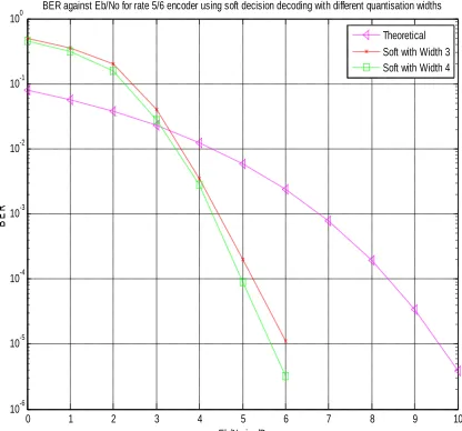
Using configurable rate of 5/6 as shown in figure9 for 3 and 4-bits quantization widths using soft decision decoding,this rate obviously presents us with the best performance compared with the previous rates discussed earlier. The Bit Error Rate curves at

10-5BER for 3-bit quantization measured a coding gain of 3.4dB

while that of 4-bit quantization has 3.3dB coding gain. This does not show any significant difference. Still leaving the data

sequence at 1 million bits and a range of 0 –10dB SNR to get a

better BER performance, a simulation was carried out using a less number of bit sequence of a hundred thousand (100,000) bits, we observed that reducing the data sequence while keeping the SNR range the same reduces the BER performance when

taken at the same value (say 10-5BER) though the computational

speed tends to increase. Therefore, in order to get a better BER performance, the computational speed is traded off for both lower and higher code rates.

0 1 2 3 4 5 6 7 8 9 10

10-6 10-5 10-4 10-3 10-2 10-1 100

Eb/No in dB

BER against Eb/No for rate 2/3 encoder using soft decision decoding with different quantisation widths

Theoretical Soft with Width 2 Soft with Width 3 Soft with Width 4

0 1 2 3 4 5 6 7 8 9 10

10-6 10-5 10-4 10-3 10-2 10-1 100

Eb/No in dB

Fig-9: BER performance of configurable rate 5/6 convolutional encoder showing curve for 3-bit and 4-bit quantization widths with soft decision decoding.

Table1 below shows a summary of the comparison of the whole coding gains as obtained for the different rates at different quantization bit levels of the performed soft and hard decision decoding.

Table 1: Summary of the coding gains

V. CONCLUSION

This paper have carefully covered modeling of configurable rate convolutional encoder with Viterbi decoder from a mother code rate 1/2 and a constraint length 7 convolutional code from which other higher rate of 2/3, 3/4 and 5/6 were further obtained with each exhibiting a low performance degradation when compared with the mother code. From the analysis of this work, our observations have proved that in using Viterbi decoder to

decode the normal ‘1/n’ code rate with K constraint length, a

trace-back length of ‘Kx5’ or ‘Kx6’ will be fully enough for the

Viterbi decoder to comfortably handle the received data symbol decoding without any noticeable performance degradation as against when comparison is made with a Viterbi decoder with an infinite memory.

REFERENCES

[1] R.W. Lucky, “A survey of the communication theory

literature; 1968-1973” IEEE Trans inform. Theory, Vol. IT-19,

pp. 725-739, Nov. 1973

[2] Forney, G.D and Ungerboeck, G, “Modulation and Coding for Linear Gaussian Channels, “IEEE Trans. Inform. Theory, Vol. 44, No.6, pp.2384-2415, oct.1999.

[3]. W. Chen. (2006), ‘RTL Implementation of Viterbi Decoder’, MSc. Thesis, Linköpings University

[4].KE-Lin Du and M. Swamy, Wireless Communications Systems: From RF Subsystems to 4G Enabling Technologies, Cambridge University Press, 2010.

[5] C. E. Shannon: "A mathematical theory of communication,"

Bell System Technical Journal, vol. 27 ,October 1948, pp. 379–

423

[6] C. Berrou, A. Glavieux and P. Thitimajshima, “Near

Shannon Limit Error-Correcting Coding and Decoding:Turbo

codes”, ICC’ 93, Conference Record, Geneva, pp. 1064–1070, 1993

[7]. Theoddore S. Rappaport “Wireless communications principle and practice”, Second edition, Prentice Hall, 2002. [8]. Branka Vucetic, “An Adaptive Coding Scheme for Time -Varying Channels”, IEEE Trans. Commun., vol. COM-39, pp. 653-663, May 1991.

[9]Wikipedia,(2010) 4G [Available at:

http://en.wikipedia.org/wiki/4G] [Viewed on June 3, 2014].

0 1 2 3 4 5 6 7 8 9 10

10-6 10-5 10-4 10-3 10-2 10-1 100

Eb/No in dB

BER against Eb/No for rate 5/6 encoder using soft decision decoding with different quantisation widths Theoretical Soft with Width 3 Soft with Width 4

Code

rate

Soft

decision

with

2-bits

Soft

decision

with

3-bits

Soft

decision

with

4-bits

Hard

decision

with

1-bit

1/2 4.20dB 5.30dB 5.35dB 3.2dB

2/3 3.90dB 4.25dB 4.28dB

-3/4 3.40dB 4.0dB 4.0dB

-[10].http://www.1core.com/library/comm/viterbi/viterbi.pdf

“Viterbi Algorithm for Decoding of Convolutional Codes”. 1 -CORE Technologies, November, 2008.

BIOGRAPHY

Engr. Ogbonna A. Ekwe is a highly motivated Electronic Engineer with a bias in Communications. He obtained his Bachelor of Engineering (B.Eng.) degree in Electronics Engineering at the University of Nigeria, Nsukka in 2005, and a

Master’s Degree in Electronic Communications and Computer

Engineering from University of Nottingham, United

Kingdom in 2011. He is a member of Institute of Engineers and Technology (IET), Nigerian Society of Engineers (NSE), Council for the Regulation of Engineering in Nigeria (COREN). He possesses many years of experience in different work environments with excellent team leadership qualities. Ekwe, O. A is presently lecturing in the department of Electrical/Electronic Engineering, Michael Okpara University of Agriculture, Umudike, Abia State, Nigeria. His research interest are in the areas of Interference management for cellular communication, Communication techniques for next generation cellular systems, Channel fading mitigation for fixed and mobile wireless communication systems, etc.

Iroegbu Chibuisi received his B.Eng. degree in Electrical and Electronics Engineering from Michael Okpara University of Agriculture, (MOUAU) Umudike, Abia State Nigeria in 2010, and currently doing a Master of Engineering degree in Electronics and Communication Engineering, Michael Okpara University of Agriculture, (MOUAU) Umudike, Abia State Nigeria. He is a member of International Association of Engineers. His research interests are in the fields of wireless sensor networks, Electronic and Communication Systems design, Security system design, Expert systems and Artificial Intelligence, Design of Microcontroller based systems, Channel coding etc

Okoro Kalu Christopher received his B.Eng. degree in Electrical and Electronics Engineering from Madonna University, Nigeria in 2008, a

master’s degree in Power System Engineering,

University of Lagos, Nigeria in 2013. and currently doing a Phd in the department of Electrical and Electronics Engineering, Michael Okpara University of Agriculture, Umudike, Abia State Nigeria. He is a member of Institute of Electrical and Electronics Engineers. Okoro K. C is presently lecturing in the department of Electrical/Electronic Engineering, Michael Okpara University of Agriculture,