Experimental Study and Optimization of Reaction
Kinetics in Gypsum Calcination
Mr. Govinda V. Late1, Dr. P.V. Thorat2, Prof. R. S. Jadhao3
1Mr. Govinda V. Late1, Department of Chemical Engineering (C.O.E.T.Akola, India),
2Dr. P.V.Thorat2, Department of Chemical Engineering (C.O.E.T.Akola, India),
3Prof. R.S. Jadhao3, Department of Chemical Engineering (C.O.E.T.Akola, India),
Abstract: Gypsum (calcium sulphate dihydrate) is of great industrial importance with over 95,000 ktonnes being used in the world per annum. The greatest use of gypsum is in the production of plaster (calcium sulphate hemihydrate) for use as an interior finisher. Plaster is produced by the calcination (thermal decomposition) of gypsum.
There are a number of different phenomena occurring within a calciner, including heat transfer, mass transfer, particle and gas mixing, elutriation and the dehydration reaction itself. All these processes interact with each other. Although a lot of research has been carried out in these areas already, the literature has been found to contain significant discrepancies. This study contains experimental work which has been carried out in order to better understand the physical processes occurring within a gypsum calciner. The rate of dehydration of gypsum (35-67μm in diameter) has been studied in a fluidized bed reactor.
Experiments were carried out at bed temperatures of 100 to 170°c. The fluidizing gas was air with water vapour pressures of 0.001 to 0.30 atm. The dehydrations were under differential conditions. A study of the fluidisation and elutriation properties of gypsum in batch vessels (cylindrical and conical) has been carried out. The mechanics of elutriation has been investigated and modeled for various freeboards, superficial gas velocities and air humidities. Residence time distributions were elucidated. Finally, the above experimental data and component models have been investigated for their applicability to producing a model of the laboratory scale gypsum calciner.
Keywords: gypsum, calcination, plaster, fluidization, modelling, nucleation
I. INTRODUCTION
This paper studies the chemical and physical processes in the industrial production of plaster from gypsum. Gypsum is the common name for calcium sulphate dihydrate, CaSO4.2H20. Plaster is the common name for dehydrated gypsum. Plaster is composed of a
mixture of the different calcium sulphate phases, including calcium sulphate hemihydrate, CaSO4. 1/2H20 and calcium sulphate
anhydrite, CaSO4. The aim of the work undertaken in this seminar is to improve the understanding of the processes occurring during the calcination (thermal decomposition) of gypsum to produce plaster in a conical kettle calciner. An experimental study of the dehydration kinetics of gypsum in a fluidised bed reactor;
A. Gypsum…?
Gypsum is the common name for calcium sulphate dihydrate, CaSO4.2H20. Since the 1980's there has been a large increase in the production and use of synthetic gypsum [Bennet, 1998]. Synthetic gypsum is formed as a by-product of several industrial processes. The main sources are from flue gas desulphurisation (DSG gypsum) and the production of wet phosphoric acid from phosphate rock (phosphogypsum). Greater quantities of phosphogypsum are produced than any other synthetic gypsum; however they are hard to market because of the high levels of impurities, including radioactive elements [Roskill, 1997].
B. Gypsum Dehydration Sequence
Plaster is produced from the dehydration of gypsum. The calcium sulphate dehydrate dehydration sequence is shown in Figure 1.1. Calcium sulphate dihydrate (hereafter referred to as dihydrate) dehydrates on heating to calcium sulphate hemihydrate (hereafter referred to as hemihydrate). Hemihydrate can exist as β and αform. The β-hemihydrate is produced by dry calcination and is the
main constituent of plaster. The α-hemihydrate is produced by wet calcination at elevated pressures or atmospheric pressure with the
ambient conditions and will readily rehydrate to hemihydrate in the presence of water vapour. All is stable at ambient conditions and Al is not stable below 1180°C.
C. Calcination..?
“Thermal treatment to effect a decomposition, phase transition or removal of a volatile fraction” Calcination is carried out in furnaces or reactors (sometimes referred to as Kiln or calciners) of various design including Shaft Furnaces, Rotary kilns, Multiple hearth furnaces and fluidized bed reactors.
D. Objectives of Calcination
1) Maximize rehydratable material to add strength to board core;
2) Stabilizing Stucco phases will allow some stabilization of water gauge
3) Core Cementitious Gypsum is directly proportional to Bond Strength.
E. The Chemistry of the CaSO4-H20 system
The CaSO4-H20 system is characterised by five solid phases, four of which can exist at ambient conditions. The fifth phase, Anhydrite I, exists only at temperatures in excess of 1180°C [Wirsching, 1990]:
1) Calcium Sulphate dihydrate ; CaSO4.2H20 : Dihydrate, D
2) Calcium Sulphate hemihydrate : CaSO4.1/2H20 : Hemihydrate, II
3) Calcium Sulphate Anhydrite III : CaSO4: Anhydrite III, AIII
4) Calcium Sulphate Anhydrite II: CaSO4: Anhydrite II, AII
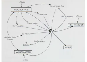
Figure 1.2: Basic influence diagram for the calciner.
F. Phase Analysis
Phase analysis allows the differentiation between the dihydrate, hemihydrate and anhydrite forms of calcium sulphate. Analysis techniques must be carried out immediately after sample production as AIII is metastable at ambient conditions. In the presence of water vapour it reverts back to hemihydrate. Also, the hemihydrate phase will readily absorb up to 2% of its own weight of water vapour without transforming to dihydrate. This water can be completely removed by heating at 40°C.
The analysis of the separate phases has been attempted by many experimenters. Techniques used include proximate analysis (PA), X-ray diffraction (XRD), infra-red spectroscopy (IRS), microscopy, calorimetry, differential thermal analysis (DTA) and gravimetric thermal analysis (TGA). These techniques have been used qualitatively rather than quantitatively.
G. Proximate Analysis (PA)
Proximate analysis is a relatively simple technique involving hydrating, heating and weighing samples in order to deduce the phase composition. The results of this technique are quoted to 0.1 %, however it is stressed that this is not the true precision. A sensitivity of 1-5%, depending upon the experience of the analyst, is probably more reasonable. The great advantage of this technique for phase analysis is that a large number of samples can be analyses simultaneously.
The decomposition reactions occur at different temperatures, as shown in Table 2.3
[image:4.612.182.430.546.703.2]II. METHODOLOGY / CALCULATIONS
A. Calculation of Fluidisation Properties
1) Calculation of Minimum Fluidisation velocity, Umf: The minimum fluidisation velocity, Umf in m/s, can be calculated from the
Carman-Kozeny Equation for spherical particles [Coulson & Richardson, 1991]:
… (2.1) Where Umf= minimum fluidising velocity, m/s
g = 9.81 m/s2, εB = Bed Voidage
TB = Bed Temperature (0C),ρg = Gas density (kg/m3)
μ = Gas viscosity (kg/m.s)
dp = Average gypsum particle size (m)
ρs = gypsum density (kg/m3),φs = Shape factor
The minimum fluidisation velocity at the conditions described above has been calculated at 0.496 cm/s (0.004964916 m/s). The
calciner operates in the region of 0.12 m/s; i.e. around 30 times the estimated umf
2) Calculation of Minimum Bubbling Velocity, Umb: The minimum bubbling velocity, Umb, can be calculated from the
Abrahamsen-Geldart Correlation [Pell, 1990]:
…… (2.2) Where Umb = the minimum boiling fluidising velocity (m/s);
F = the fraction of solids which are less than 45 microns For the conditions above, Umb has been calculated to be approximately twice the minimum fluidising velocity. Therefore the calciner will exist in a `bubbly' region.
3) Calculation of Terminal Velocity, U*t : For spherical particles with a particle Reynolds number of less than 0.4 it can be
assumed that the terminal velocity can be calculated from Stokes law [Pell, 1990]. Therefore:
….. (2.3)
Where Ut = the particle terminal velocity (m/s);
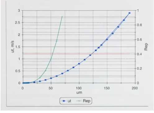
Figure 2.1: Calculation of ut and rep
Figure 2.1.Shows the calculation of Ut and Rep for different size particles. As can be seen, the particle Reynolds number is close to the limit of 0.4 for decent accuracy. Therefore a more detailed method for calculating the terminal velocity, which also takes into account the shape factor of the particles. The equation below gives the terminal velocity as [Haider and Levenspiel, 1989]:
…. (2.4) Where dp* = dp[{ρg (ρs- ρg) g}/μ^2]^1/3
4) Calculation of Superficial gas velocity, u0 (m/s): In the simplest sense elutriation occurs when the superficial gas velocity
within the bed exceeds a particle terminal velocity. It is measure of the calculation of Dispersion Coefficient (D) and Dispersion Number.
The superficial gas velocity is being calculated by using the below formula as,
=
( )∗ ………. (2.5)
B. Calculation of Heat Transfer Properties
It is apparent that the dehydrations are not limited by heat and mass transfer external to the particles. It is also apparent that the temperature, water vapour pressure and particle size have an effect upon the rate of dehydration. However it is also important to consider whether heat and mass transfer inside the particles is limiting the rate of dehydration. This was investigated by setting up a series of models to describe these transfer processes inside the particles.
1) Calculations of Internal Heat transfer coefficient: The internal heat transfer coefficient is being calculated by using the
following correlation of Nusselt Number as;
……(2.6)
2) Calculation of Outside Heat transfer coefficient (ho or hmax) : For the calculation of Outside heat transfer coefficient (ho) for gas
solid system apparent density of the gypsum particle is very important and is being taken into consideration.
….. (2.7)
3) Calculations of Overall heat transfer coefficient : The Overall heat transfer coefficient (U) for gas solid system in W/m2K will be calculated as
…… (2.8) Where U= overall heat transfer coefficient;
4) Heat Transfer area calculations: Here we have mainly make the calculation of the overall heat transfer coefficient by calculating the internal and external heat transfer coefficient and using the below equation as;
Formula: Q= U*A*ΔT……… (2.9) Where,
U= Overall heat transfer coefficient
A= Heat transfer area
ΔT = Log mean temperature difference
Q= Heat supplied to the chamber
Q value is taken from multi-chamber calciner model
Heat supplied to the chamber (Q) = m*Cp*ΔT… (2.10)
Here now we have calculated the Number of tubes required in the given chamber from the above calculated Heat transfer area. We have check here that from number of tubes whether calculated area is less than the Maximum Possible area.
Now the surface area of one tube is calculated as, Surface area of one tube = 2*π*ro*l……… (2.11) Where l = Length of one tube after clearance (m); ro = Outside radius of one tube (m).
No.of tubes required, N = … (2.12)
For the diameter of the tube from which we have calculate the required Heat transfer area and number of tubes required, by using the same diameter of the tube we have make calculate the maximum possible area and maximum possible number of tubes required. We have calculate tubes by two sides as
Tubes along the length, Tubes along the width. Where
Tubes along length = ( )
( )
Tubes along width = ( . )
( )
Therefor after getting the tubes on both the sides we have calculate the maximum possible number of tubes in the given chamber by multiplying the tubs along length and tubes along width.
Note: As the maximum possible tubes are more than the required number of tubes, maintaining the temperature is feasible.
C. Calculation of Kinetic properties
The above reaction is a typical calcination reaction which is carried out in the fluidised bed reactor in which the volatile fraction i.e 1.5 molecules of water are removed from the combined water molecule. In the above reaction we see that there are four phases exist and combinly we called it as STUCCO. Here we analyse the each phase with the help of moisture content which has been determined by the proximate analysis method.
1) Calculation of Activation Energy and Order of Reaction: Once the mechanism has been decided upon the other kinetic
parameters can be calculated. In general the rate constant of a solid state reaction increases with temperature according to an exponential law (Arrhenius equation):
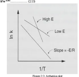
[image:8.612.158.435.396.666.2]k = A*e -E/RT……… (2.13)
Figure 2.2: Arrhenius plot
According to Jim flether-Sion Study thesis, Arrhenius plots will be drawn and the activation energy, E and frequency factor, A
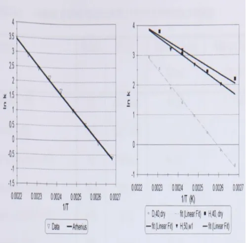
Phosphogypsum. Figure 2.4 demonstrates the difference between the Arrhenius plots for gypsum and hemihydrate. The hemihydrate plot has a lower gradient and a lower intersect than the gypsum plot.
Figure 2.3: typical Arrhenius plot for 40 µm phosphogypsum; Figure 2.4: comparison of dry Arrhenius plot, hemihydrate and dihydrate;
A series of reactions at different temperatures are carried out with all the remaining experimental conditions constant. Reaction rate constants can then be determined for each temperature. An Arrhenius plot of Ink versus l/T (K) allows the activation energy, E, and frequency factor A, to be calculated from the gradient and intersect as shown in Figure 2.2.
2) Residence Time Calculations: In order to apply information from kinetic studies of the dehydration of gypsum to the calciner it is necessary to be able to model the residence time distribution of particles in the vessel. A better understanding of the solids mixing inside the kettle is required in order to develop a model of the calcination system. The extent of mixing within the kettle can be evaluated using a tracer test to elucidate the residence time distribution (RTD) of particles in the system.
Residence time is calculated by knowing the superficial gas velocity and dispersion number, Bed Weight and solid flow rate,
tmean (hr.) =
, ( )
, ( / )……… (2.14)
III. CONCLUSIONS AND FUTURE WORK
Although a lot of research has been carried out on fluidisation, the difference between theoretical models and experimental research has been found to vary by as much as several orders of magnitude. Therefore an experimental study has been carried out into the fluidisation properties of phosphogypsum. Particular emphasis has been placed on the elutriation of phosphogypsum as the superficial velocity in the kettle has been calculated to be greater than the terminal velocity of the majority of the particles in the bed.
A model has been developed which give the overall reaction rate under different conditions of water vapor pressure and temperature. It was found that particle size was not a significant factor for the gypsum particles studied. Therefore the local reaction rate in a gypsum calciner can be predicted given the operating conditions.
To summarise, it is recommended that the following further work is carried out
A. Studies into the dehydration kinetics of other sources of gypsum (synthetic and mined).
B. Investigations into the AIII to HH rehydration reaction at high water vapor pressures.
[1] Sion Cave, 2000, Gypsum Calcination In A Fluidised Bed Reactor, 1-222. [2] Fogler, S. 1986, Elements of Chemical Reaction Engineering.
[3] Donald Q. Kern’s, Process Heat Transfer, International Edition-1965, 675-714.
[4] Paper on Fluidized behaviour and heat transfer in a bubbling fluidized bed incinerator by “Ming-Yen Wey,1,* Chiou-Liang Lin2 and Shr-Da You1” [5] Coulson, J., M.; Richardson, J., F., Chemical Engineering- Volume 2, Fifth Edition-2002 315-332, PergamonPress. Oxford.
[6] Hensen, F., E.; Clausen, H., 1973, Dehydration of Gypsum. Zem. Kalk. Gips., 26(5) 223-226. GERMAN. [7] The Canadian Journal of Chemical Engineering, Vol. 53, A@& 1975
[8] Green, R., H., (ed), 1984, Perry's Chemical Engineers' Handbook, 6th ed section 5,6 and 7, McGraw-Hill, London. [9] Levenspiel, Octave, Chemical reaction engineering/Octave Levenspiel. - 3rd ed.1999, 293-312 and 566 -589.
[10] Determination of heat transfer coefficients in a fluidized bed at variable flow velocity Journal, Journal of engineering physics Volume 10, Issue 2 ,pp 107-109. [11] Kroschwitz, J., I., 1992, Kirk-Othmer Encyclopedia of chemical technology, Wiley, Chichester.
[12] Kunii, I.; Levenspiel, O., 1991, Fluidisation Engineering, 2nd ed, Butterworth-Heinmann, London.
[13] Warren L. McCabe, Julian C. Smith, Peter Harriott, Unit Operations of Chemial Engineering/-5thed 1993, 285-329
[14] Kreith, F., and Bohn, M., S., 1997, Principles of Heat Transfer, 5th Edition, PWS Publishing Company, London. [15] Coulson, J., M.; Richardson, J., F., 1971, Chemical Engineering- Volume 3, PergamonPress. Oxford.
[16] Roskill Information Services Ltd, 1997, The Econmics of Gypsum and Anhydrite 1997, seventh edition, reproduced in Gypsum, Lime and Building Products, November 1997, 30-34.
[17] Saxena, S., C., and Mathews, A., 1984, ChemEng Science, 39 917.
[18] Venkatesh D., R., Chaouki, J and Kivana, D. 1996, Powder Technology. 89.179-186.
[19] Deo Karan Ram., International Journal of science and Research (IJSR), Indian Online ISSN: 2319-7064, vol 2, issue 2, February2013.