Density Functional Theory Embedding for Correlated Wavefunctions

(1)

for Correlated Wavefunctions

Thesis by

Jason D. Goodpaster

In Partial Fulfillment of the Requirements

for the Degree of

Doctor of Philosophy

California Institute of Technology

Pasadena, California

2014

(2)

c

2014

Jason D. Goodpaster

(3)

(4)

Acknowledgments

It is with immense gratitude that I acknowledge the support and help of my thesis

advisor Professor Thomas F. Miller III. His encouragement, enthusiasm, and guidance

was invaluable throughout my Ph.D. He has taught me how to develop interesting

questions and how to approach answering them. He has made me a better scientist,

theorist, and communicator. I truly cannot imagine a better advisor and mentor for

my graduate studies.

Additionally, I would like to thank the faculty of the Division of Chemistry and

Chemical Engineering. In particular, I thank my thesis committee, Dr. William

Goddard III, Dr. Zhen-Gang Wang, and Dr. Mark Davis for their support, scientific

discussions, and guidance in my future career. I am also deeply grateful to the

late Aron Kuppermann for his elegant presentation of quantum mechanics, constant

encouragement, and his friendly late night discussions while we were “burning the

midnight oil”.

I also must thank the division administrative staff, Priscilla Boon for all the

sup-port she has provided to myself and the Miller Group, Kathy Bubash for her

ad-ministrative expertise, and Tom Dunn, Zailo Leite, and Naveed Near-Ansari for their

technical expertise, specifically with computing.

I thank all the members of the Miller group: Bin, Nick, Nandini, Romelia, Artur,

Josh, Connie, Taylor, Mike, Fran, Kuba, Frank, Michiel, Joonho, Mark, and Matt.

Thank you all for your scientific discussion, help with coding and computing, and

encouragement. It was truly an honor to work with you all.

(5)

through-out graduate school; you were always there for me. I thank my friends for their

understanding, encouragement, and for making my graduate school experience more

enjoyable.

Lastly, thank you Julia. You challenge me to be a better scientist and person, you

support me in all my endeavors, and you encourage me to strive above and beyond.

(6)

Abstract

Methods that exploit the intrinsic locality of molecular interactions show significant

promise in making tractable the electronic structure calculation of large-scale

sys-tems. In particular, embedded density functional theory (e-DFT) offers a formally

exact approach to electronic structure calculations in which the interactions between

subsystems are evaluated in terms of their electronic density. In the following

disser-tation, methodological advances of embedded density functional theory are described,

numerically tested, and applied to real chemical systems.

First, we describe an e-DFT protocol in which the non-additive kinetic energy

component of the embedding potential is treated exactly. Then, we present a general

implementation of the exact calculation of the non-additive kinetic potential (NAKP)

and apply it to molecular systems. We demonstrate that the implementation using

the exact NAKP is in excellent agreement with reference Kohn-Sham calculations,

whereas the approximate functionals lead to qualitative failures in the calculated

energies and equilibrium structures.

Next, we introduce density-embedding techniques to enable the accurate and

sta-ble calculation of correlated wavefunction (CW) in complex environments.

Embed-ding potentials calculated using e-DFT introduce the effect of the environment on

a subsystem for CW calculations (DFT). We demonstrate that

WFT-in-DFT calculations are in good agreement with CW calculations performed on the full

complex.

We significantly improve the numerics of the algorithm by enforcing orthogonality

(7)

projection-based embedding scheme, we rigorously analyze the sources of error in quantum

embedding calculations in which an active subsystem is treated using CWs, and the

remainder using density functional theory. We show that the embedding potential

felt by the electrons in the active subsystem makes only a small contribution to the

error of the method, whereas the error in the nonadditive exchange-correlation energy

dominates. We develop an algorithm which corrects this term and demonstrate the

(8)

List of Figures

1.1 Accuracy in the extrapolation of kinetic energy from the ZMP method 15

1.2 The 2s electron density for an isoelectronic series of atoms calculated

using KS-DFT and e-DFT . . . 17

1.3 The KSCED effective potential for an isoelectronic series of atoms . . . 21

1.4 The NAKP, KSCED effective potential, and the 2s electron density for the modified NAKP . . . 25

2.1 The water dimer dissociation curve obtained using KS-DFT and e-DFT 43 2.2 Basis set dependence of the water dimer dissociation curve obtained using KS-DFT and e-DFT . . . 45

2.3 The Li+-Be dissociation curve obtained using KS-DFT and e-DFT . . 46

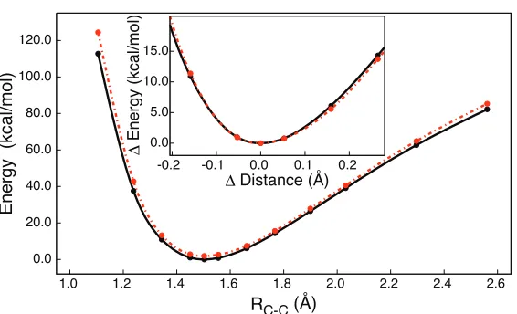
2.4 The CH3-CF3dissociation curve for heterolytic cleavage of the C-C bond obtained using KS-DFT and e-DFT . . . 48

2.5 Symmetric dissociation curves for the water trimer, illustrating the pair-wise additivity of the NAKP. . . 51

2.6 Wall-clock timings for lattices of hydrogen molecules . . . 53

2.7 Error in the total energy of e-DFT relative to KS-DFT for lattices of hydrogen molecules . . . 54

3.1 An illustrative Newton step in the OEP calculation . . . 75

3.2 WFT-in-DFT embedding for the ethylene-propylene dimer. . . 77

3.3 DFT-in-DFT embedding for the hexaaquairon(II) cation. . . 80

(13)

3.5 CCSD(T)-in-DFT embedding for the hexaaquairon(II) cation. . . 85

4.1 Contributions to the total WFT-in-DFT error . . . 103

4.2 MP2 corrected WFT-in-DFT errors . . . 106

4.3 Potential energy surface for 1-penten-1-one . . . 108

4.4 Error in dissociation of F− from alkane chain . . . 110

4.5 Error in dissociation of F− from alkene chain . . . 112

4.6 Error in exchange reaction energy for alkane and alkene chains . . . 114

(14)

List of Tables

1.1 Total energy and ionization energy obtained using KS-DFT and e-DFT. 20

1.2 Total energy and ionization energy obtained using e-DFT with the NAKP

switching function . . . 24

3.1 High-spin/low-spin splitting energies in cm−1 for the hexaaquairon(II) cation using MP2 theory and MP2-in-DFT . . . 84

3.2 High-spin/low-spin splitting energies in cm−1 for the hexaaquairon(II) cation using CCSD(T) theory and CCSD(T)-in-DFT . . . 86

4.1 CCSD(T) reaction energies and barriers in the test set . . . 102

4.2 Change in the dipole moment for dissociation of F− from the alkane and

(15)

Summary

Quantum-chemistry calculations invariably feature a compromise between

computa-tional efficiency and accuracy. Kohn-Sham Density Funccomputa-tional Theory (KS-DFT) is

one of the most commonly used methods because it is tractable for systems

contain-ing up to a thousand atoms. However, DFT methods, which generally employ

ap-proximate descriptions of electron correlation, often fail to even qualitatively predict

reaction barriers, which are critical in determining reaction rates and mechanisms.

More rigorous correlated wavefunction (CW) methods can provide an accurate and

systematically improvable description of reaction barriers, but poor scaling of these

methods can lead to impractical computation costs for systems with even tens of

atoms.

Embedded density functional theory (e-DFT), is a formally exact approach to

electronic structure, which exploits the locality of molecular interactions. In the

e-DFT approach, a system is divided into smaller subsystems. Then, the interactions

between subsystems are evaluated in terms of their electronic density. This approach

naturally leads to two different partitioning schemes. One, a large system can be

sep-arated into many smaller subsystems, allowing for significant computational savings

as this leads to a naturally parallelizable algorithm. Two, a large system is

sepa-rated into a ‘high-level’ (accurate) and a ‘low-level’ (approximate) regions; therefore,

if higher accuracy is required for a region of system, a higher level of theory can

be seamlessly embedded into a DFT environment and still remain computationally

tractable as only a handful of atoms are treated at the CW level. The objectives of the

(16)

frag-mentation schemes; however, e-DFT avoids the uncontrolled approximations (such as

link atoms) and errors associated with subsystem interfaces that fundamentally limit

other widely used methods.

This dissertation is focused on the development of new methods that make e-DFT

an accurate, practical, and scalable method for the description of complex systems.

The following key contributions are discussed: (i) the development of numerically

exact methods for obtaining subsystem embedding potentials in e-DFT, which reduce

embedding errors by orders of magnitude in comparison with previously available

approximate methods, (ii) the development of parallelization algorithms that enable

the description of large systems with sub-linear scaling of the required computational

time, (iii) the combination of e-DFT potentials with correlated wavefunction theory

(WFT) methods to enable seamless WFT-in-DFT embedding for general systems,

and (iv) the development of systematically improvable methods for WFT-in-DFT to

allow for a hierarchy of embedding methods with increasing accuracy.

In Chapter 1, we describe an embedded density functional theory (DFT)

proto-col in which the non-additive kinetic energy component of the embedding potential

is treated exactly. At each iteration of the Kohn-Sham equations for constrained

electron density, the Zhao-Morrison-Parr constrained search method for constructing

Kohn-Sham orbitals is combined with the King-Handy expression for the exact kinetic

potential. We use this exact embedding protocol to calculate ionization energies for

a series of 3- and 4-electron systems, and the results are compared to embedded DFT

calculations that utilize the Thomas-Fermi (TF) and the Thomas-Fermi-von

Wei-sacker approximations to the kinetic energy functional. These calculations illustrate

a breakdown due to the TF approximation for the non-additive kinetic potential, with

errors of 30-80% in the calculated ionization energies; by contrast, the exact protocol

(17)

N. Ananth, F. R. Manby, and T. F. Miller III, “Exact non-additive kinetic potentials

for embedded density functional theory,” J. Chem. Phys., 133, 084103 (2010). In Chapter 2, we present a general implementation of the exact calculation of

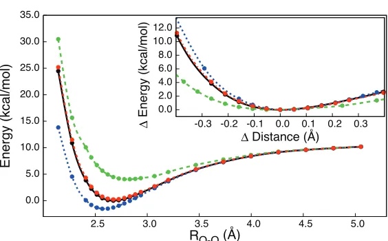
the non-additive kinetic potential (NAKP). Potential energy curves are computed

for the dissociation of Li+-Be, CH3-CF3, and hydrogen-bonded water clusters, and

e-DFT results obtained using this exact treatment of the NAKP are compared with

those obtained using approximate kinetic energy functionals. In all cases, the exact

NAKP is in excellent agreement with reference Kohn-Sham calculations, whereas the

approximate functionals lead to qualitative failures in the calculated energies and

equilibrium structures. We also demonstrate an accurate pairwise approximation to

the NAKP that allows for efficient parallelization of the method in large systems;

benchmark calculations on molecular crystals reveal ideal, size-independent scaling

of wall-clock time with increasing system size. This work has been published as J.

D. Goodpaster, T. A. Barnes, and T. F. Miller III, “Embedded density functional

theory for covalently bonded and strongly interacting subsystems,” J. Chem. Phys.,

134, 164108 (2011).

In Chapter 3, we introduce density embedding techniques to enable the

accu-rate and stable calculation of CWs in complex environments. Embedding potentials

calculated using e-DFT introduce the effect of the environment on a subsystem for

wavefunction calculations (WFT-in-DFT). These methods are demonstrated for

cal-culating the potential energy curve of the dispersion-bound ethene-propene dimer

and for the hexaaquairon(II) ion (HA). The potential energy curve for the

ethene-propene dimer reveals that benchmark CCSD(T) calculations performed over the full

complex can be reproduced within 0.05 kcal/mol using this method, illustrating that

small energy differences can be accurately calculated while embedding across a

cova-lent bond. e-DFT calculations on HA that employ these new techniques demonstrate

(18)

the high-spin states. The ability of different exchange-correlation (XC) functionals to

describe the energy differences between the low-spin and the high-spin states (∆ELH)

and to describe the ligation energy in HA is studied. KS-DFT calculations of ∆ELH

demonstrate a strong dependency on XC functionals where WFT-in-DFT

calcula-tions reveal a significantly diminished dependency and that ∆ELH is in good

agree-ment withab initio calculations performed on the full complex. The ligation energies

have a small dependency on the XC functional and are near identical for KS-DFT

and WFT-in-DFT demonstrating that the interactions energies between subsystems

remain at DFT level accuracy. This work has been published as J. D. Goodpaster, T.

A. Barnes, F. R. Manby, and T. F. Miller III, “Density functional theory embedding

for correlated wavefunctions: Improved methods for open-shell systems and transition

metal complexes,” J. Chem. Phys., 137, 224113 (2012).

In Chapter 4, we present continuing work on projection based embedding. The

original formulation has been published as F. R. Manby, M. Stella, J. D. Goodpaster,

and T. F. Miller III, “A simple, exact density-functional-theory embedding scheme,”

J. Chem. Theory Comput., 8, 2564 (2012) and T. A. Barnes, J. D. Goodpaster,

F. R. Manby, and T. F. Miller III, “Accurate basis set truncation for wavefunction

embedding,” J. Chem. Phys., 139, 024103 (2013). Building upon that work, we analyze the sources of error in quantum embedding calculations in which an active

subsystem is treated using CW methods, and the remainder using DFT. We show

that the embedding potential felt by the electrons in the active subsystem makes only

a small contribution to the error of the method whereas the error in the nonadditive

exchange-correlation energy dominates. We test an MP2 correction for this term

and demonstrate that the corrected embedding scheme accurately reproduces the

full wavefunction calculations for a series of chemical reactions. This work has been

(19)

“Accurate and systematically improvable density functional theory embedding for

(20)

Chapter 1 Exact non-additive kinetic potentials for embedded

density functional theory

1.1 Introduction

Orbital-free embedded density functional theory (e-DFT) is an appealing method

for calculating the electronic structure of complex molecular systems. It provides a

formally exact framework for dividing the total electronic density of a system into

subsystem densities that can be separately calculated.1–4This feature of e-DFT allows for the development of multiscale strategies in which the electronic density for regions

of central interest is calculated with high accuracy, while the electronic density for

surrounding regions is obtained using more approximate techniques.5–7

However, in addition to the usual approximations for the basis set and the

exchange-correlation functional that appear in Kohn-Sham (KS) DFT,8 e-DFT requires the evaluation of a non-additive contribution to the kinetic energy from the subsystem

densities.4 This term, which is generally largest for cases in which the subsystem densities are strongly overlapping,9 is a significant source of error in many e-DFT calculations, and it currently limits the method to applications in which the

subsys-tem densities involve non-bonded or weakly interacting molecular groups.4,9Although encouraging progress towards the accurate calculation of the non-additive kinetic

(21)

energy contribution in e-DFT calculations, and we report calculations in which the

protocol is applied to 3- and 4-electron systems that exhibit strongly overlapping

subsystem densities. Although, in its numerically demonstrated form, this protocol

does not offer any computational speed-up over the KS calculation for the full system,

it suggests new methods to systematically, efficiently, and accurately perform e-DFT

calculations for large systems, which we discuss.

1.2 Orbital-Free Embedded DFT

Suppose that the entire electronic density ρAB for a closed-shell system is divided

into two subsystems, ρA and ρB, such that ρAB=ρA+ρB. The one-electron orbitals

that give rise to these subsystem electronic densities obey the coupled Kohn-Sham

equations for constrained electron density (KSCED),4

−1

2∇

2₊_VKSCED

eff [ρA, ρB;r]

φA_i (r) = A_i φA_i (r), i= 1, ..., NA

2 , (1.1)

−1

2∇

2₊_VKSCED

eff [ρB, ρA;r]

φB_i (r) =B_i φB_i (r), i= 1, ...,NB

2 , (1.2)

where NA and NB are the number of electrons in the respective subsystems,

ρA(r) = 2

NA/2

X i=1

|φA

i (r)|

2_, _and _(1.3)

ρB(r) = 2

NB/2

X i=1

|φB

i (r)|

2_. _(1.4)

In these coupled equations,V_effKSCED[ρA, ρB;r] is the KS effective potential for

(22)

V_effKSCED[ρA, ρB;r] =vne(r) +vJ[ρAB;r] +vxc[ρAB;r] +vnad[ρA, ρB;r], (1.5)

and V_effKSCED[ρB, ρA;r] is the similarly defined KS effective potential for subsystem B

embedded in subsystem A. The contributions to the KS effective potential include

vne(r) = −

Nnuc

X i

Zi |r−Ri|

, (1.6)

vJ[ρAB;r] =

Z _ρ

AB(r0)

|r0₋_r_|dr

0_, _and _(1.7)

vxc[ρAB;r] =

δExc[ρ]

δρ

ρ=ρAB

(r), (1.8)

which are the usual nuclear-electron Coulomb potential, Hartree potential, and

exchange-correlation potential, respectively, and Nnuc is the number of nuclei in the system.

The final term in V_effKSCED[ρB, ρA;r] is the non-additive kinetic potential (NAKP)

vnad[ρA, ρB;r] =

δTnad

s [ρA, ρB]

δρA

(r) = δTs[ρ]

δρ

ρ=ρAB

(r)−δTs[ρ] δρ

ρ=ρA

(r), (1.9)

which is obtained from the functional derivative of the non-additive component of the

non-interacting kinetic energy

T_snad[ρA, ρB] =Ts[ρAB]−Ts[ρA]−Ts[ρB]. (1.10)

The total energy functional for the embedded system is

(23)

where the last three terms on the right hand side (RHS) are the nuclear-electron

Coulomb energy, Hartree energy, and exchange-correlation energy for the total

den-sity.

Two aspects of the orbital-free embedding DFT formulation are worth

emphasiz-ing. Firstly, like conventional KS-DFT, it is a theory that is exact in principle, but

practical calculations must employ an approximate form for the unknown

exchange-correlation functional. Secondly, unlike conventional KS-DFT calculations, the

em-bedding formulation introduces an NAKP because the KS orbitals for subsystem A

are not necessarily orthogonal to those of subsystem B. Without knowledge of the

exact functional for the non-interacting kinetic energy, this creates a second source of

approximation in the e-DFT approach. The significance of the NAKP is system

de-pendent, with the most severe cases including those for which the subsystem densities

ρA and ρB greatly overlap.4,9,14,15

The non-interacting kinetic energy for the density corresponding to a set of N

closed-shell orbitals is

Ts[ρ] = 2

N

X i=1

hφi| −

1 2∇

2_|φ

ii. (1.12)

Standard approximations to this kinetic energy functional include the Thomas-Fermi

(TF) result for the homogenous electron gas,16,17

TTF[ρ] =CTF

Z

ρ5/3(r)dr (1.13)

where CTF =

3 10(3π

2₎2/3_{, and the von Weizs¨}_{acker (vW) result for the limit of a}

one-electron density,

TvW[ρ] =

1 8

Z _|∇ρ

(r)|2

ρ(r) dr. (1.14)

Other approximate kinetic energy functionals can be constructed using the

(24)

PW91k kinetic energy functional10,11 employs the analytical form of the Perdew-Wang (PW91) exchange functional,19 and the TW02 functional13 and the PBE2, PBE3, and PBE4 functionals9 utilizes the form suggested by Becke.20 These func-tionals have been shown to successfully describe weakly interacting systems and

co-ordination compounds.9 Furthermore, kinetic energy functionals that have been de-veloped using linear response corrections to the homogeneous electron gas and have

been shown to work well for metals.3,21–23 However, no approximate kinetic energy functional has been demonstrated to yield accurate results for embedded subsystems

that are connected by a covalent bond.9,15,24

1.3 The Exact Non-Additive Kinetic Potential

For each iteration of the KSCED equations (Eqs. 1.1 and 1.2), {φA

i } and {φBi } (and

thusρAand ρB) are known from either the previous iteration or the initial guess, and

the NAKP must be calculated. We employ a two-step protocol to obtain the exact

NAKP. In the first step, a Levy constrained search25 (LCS) or equivalent method is used to determine the full set of orthogonal KS orbitals, {φAB

i }, that correspond to

the total density ρAB. In the second step, the NAKP is calculated from the orbital

sets {φAB

i }, {φ

A

i }, and {φ

B

i }.

1.3.1 Step 1: The Levy Constrained Search

Given a total electron density ρAB, the fully orthogonal KS orbitals {φABi } can be

calculated from an LCS, in which the non-interacting kinetic energy is minimized with

respect to one-electron orbitals that are constrained to yieldρAB.25 Alternatively, we

(25)

of KS orbitals are obtained by solving the one-electron equations " −1 2∇ 2₋ Nnuc X i Zi |r−Ri|

+V_cλ(r)

#

φ_iAB,λ(r) =iφiAB,λ(r), i= 1, ..., NAB

2 , (1.15)

where NAB=NA+NB,

V_cλ(r) =λ Z _ρ

AB(r0)−ρ˜AB(r0)

|r0₋_r_| dr

0_, _(1.16)

˜

ρAB(r) = 2

NAB/2

X i=1

|φAB

i (r)|

2_{, and} _Vλ

c (r) is a potential energy function that restrains

the ˜ρAB(r) to the target density ρAB(r). Solution of Eq. 1.15 in the limit λ → ∞ is

equivalent to performing the LCS.26–28

In practice, Eq. 1.15 is solved for six large, but finite, values of λ, and the KS orbitals and eigenvalues are obtained via extrapolation.26–28 For each value of λ, the

{λ_i}, {φAB_i ,λ}, and {∇2φAB_i ,λ} are calculated and stored on a spatial grid. For the orbitals, extrapolation to λ→ ∞ is performed via expansion to third order in 1

λ,

φAB_i ,λ(r) =φAB_i (r) + 1

λa

(1)

i (r) +

1

λ2a (2)

i (r) +

1

λ3a (3)

i (r), (1.17)

with a linear least-squares fit of the expansion coefficients{φAB

i (r), a

(1)

i (r), a

(2)

i (r), a

(3)

i (r)}

at each value ofr. The{∇2_φAB

i }are similarly obtained via extrapolation at each value

ofr, while eachi requires only a single extrapolation. With the{φABi }and{∇

2_φAB

i }

obtained on the spatial grid, the non-interacting kinetic energy for the total system

can be calculated via numerical integration using Eq. 1.12.

1.3.2 Step 2: Exact Kinetic Potentials from KS Orbitals

To calculate the NAKP from the orbital sets {φAB

i }, {φ

A

i }, and {φ

B

i }, we extend the

(26)

Minimization of the electronic energy with respect to the total electron density

ρAB yields the stationary condition8

δTs[ρ]

δρ

ρ=ρAB

(r) +vne(r) +vJ[ρAB;r] +vxc[ρAB;r] =µAB (1.18)

where µAB is a Lagrange multiplier that imposes the constraint

Z

ρAB(r)dr= NAB.

Furthermore, rearrangement of the usual KS equations yields

2

ρAB(r)

NAB/2

X i −1 2φ AB

i (r)∇

2_φAB

i (r)−iφABi (r)

2

+vne(r) +vJ[ρAB;r] +vxc[ρAB;r] = 0.

(1.19)

Comparison of these two results leads to an exact expression for the total kinetic

potential,29

δTs[ρ]

δρ

ρ=ρAB

(r) = 2

ρAB(r)

NAB/2

X i −1 2φ AB

i (r)∇

2_φAB

i (r)−iφABi (r)

2

+µAB. (1.20)

Analogous results can be derived for each of the embedded subsystems.

Specifi-cally, the electron density for subsystem A also obeys a stationary condition,2

δTs[ρ]

δρ

ρ=ρA

(r) +vne(r) +vJ[ρAB;r] +vxc[ρAB;r] +vnad[ρA, ρB;r] =µA, (1.21)

where µA is the Lagrange multiplier that imposes the constraint

Z

ρA(r)dr = NA.

Combination of Eq. 1.21 with Eq. 1.1 results in an exact expression for the subsystem

kinetic potential,

δTs[ρ]

δρ

ρ=ρA

(r) = 2

ρA(r)

NA/2

X i −1 2φ A

i (r)∇

2

φA_i (r)−A_i φA_i (r)2

+µA, (1.22)

which can be compared with kinetic potential for the total system in Eq. 1.20.

(27)

arbitrarily chosen subsystem, we likewise obtain µAB=µB, or

µA=µB. (1.23)

This result has a simple physical interpretation. In the zero temperature limit, the

Lagrange multipliers µA andµB, are equivalent to the chemical potential for the

sub-system electronic densities.8 Solution to the KSCED equations thus yields densities that are in equilibrium with respect to the number of electrons in each subsystem.

Finally, insertion of Eq. 1.20 and 1.22 into Eq. 1.9 yields the desired expression

for the NAKP,

vnad[ρA, ρB;r] =

2

ρAB(r)

NAB/2

X i −1 2φ AB

i (r)∇

2_φAB

i (r)−iφABi (r)

2

− 2

ρA(r)

NA/2

X i −1 2φ A

i (r)∇

2_φA

i (r)−

A

i φ

A

i (r)

2

. (1.24)

Note that the ZMP protocol generally yields a constant shift in the calculated set of

KS eigenenergies,{λ i};

26_{in Eq. 1.24, we see that this leads only to a constant shift in}

vnad[ρA, ρB;r] and causes no change in any calculated observables. Throughout this

study, the NAKP is shifted such that it approaches zero at large distances.

Visscher and coworkers previously observed that the NAKP can be expressed in

terms of the stationary condition for the total system (Eq. 1.18) and a subsystem

(Eq. 1.21).30 They suggested a strategy in which the ZMP method is used to ob-tain the external potentials for both the full system and the subsystem, so that the

difference between those potentials is equal to the NAKP, but this strategy has not

been implemented to our knowledge. The approach presented here directly expresses

the NAKP in terms of the KS orbitals for the total system and the subsystem (Eq.

1.24); it avoids performing the ZMP method for the subsystem, and it avoids using

(28)

is straightforward to show that Eq. 1.24 recovers the limit for weakly overlapping

subsystem densities that is reported in Ref. 30.

In another approach that does not utilize the exact framework of the KSCED

equations, Aguado and coworkers employ an embedding strategy in which the ZMP

formalism is used to constrain the sum of the subsystem densities to that of the total

density.31,32 This approach has been pursued as a useful, but approximate, strategy for partitioning a total density into subsystems.

Other e-DFT strategies also express the kinetic potential in terms of the KS

or-bitals, as we have done here. For example, Huang and Carter report an explicit

expression for the kinetic potential in terms of the KS orbitals, using the assumption

that the non-interacting kinetic energy is a linear functional of the density; an

em-pirical parameter is included in their result to account for non-linear effects.33 The approach presented here involves no adjustable parameters and no assumptions about

the linearity of the kinetic energy functional.

1.3.3 Computational Details

Calculations are performed on four atomic systems: Li, Ne7+, Q−₂_.0₅.5 and Be, where Q−₂_.0₅.5 is a model 3-electron atom that has a nuclear charge of +2.5. In all e-DFT calculations, we take ρA to be the density for a single 2s electron, and ρB includes

all other electrons. The KSCED equations for each system were solved with ρB fixed

at the density obtained from the corresponding orbitals of an unrestricted KS-DFT

calculation on the full system; this is justified for the cases studied here because

solution of the KSCED equations for ρA subject to a fixed ρB ≤ρ0 (at all r), where

ρ0 is the exact ground state density for the full system, ensures the exact calculation

(29)

1.3.3.1 Basis Sets

All calculations were performed using the fully uncontracted cc-pVTZ basis set of

Gaussian-type orbitals (GTOs),34 with only the s-type orbitals included. For calcu-lations on Q−₂_.0₅.5, the Li basis set was used. For Ne7+, the most diffuse s-orbital was removed to facilitate convergence. Although not reported, all calculations were also

repeated with slater-type orbitals, which led to somewhat improved convergence but

very similar numerical accuracy.

[image:29.612.206.446.311.484.2]

1.3.3.2 DFT Implementation Details

Figure 1.1: The difference between the non-interacting kinetic energy Ts[ρ] from

KS-DFT and from the ZMP method, plotted as a function of γ. The extrapolation is performed using {λ}={γ−jτ}, j = 5,4, . . . ,0, and using τ of 10 (red), 20 (green), and 40 (blue). See text for details.

For all applications considered here, ρA is an open shell system, and the

calcula-tions were performed using the unrestricted KS formalism. Details for the unrestricted

KSCED equations are given in the Appendix. All calculations employ the Slater

ex-change functional35 and the Vosko, Wilk, and Nusair correlation functional.36 In calculating V_effKSCED[ρA, ρB;r], a uniform radial grid is used to evaluate the

(30)

KSCED equations, the same radial grid is used to evaluate the exchange-correlation

energy and to numerically integrate the kinetic energy. For Be and Li the grid

ex-tends from r = 0 to 15, while for Q₂−_.0₅.5, r = 0 to 20 and Ne7+, r = 0 to 2. For Be, Li and Q the grid density is 2000 points/a0 and for Ne7+, 20000 points/a0. We note

that future applications that employ either a non-uniform37 or variational38 mesh will require fewer gridpoints to achieve the same level of accuracy. Unless otherwise

stated, the iterative solution of the KSCED equations were deemed converged when

the total energy of the system changed by less than 10−8 Hartrees between successive iterations.

1.3.3.3 ZMP Extrapolation

To examine the extrapolation error associated with the ZMP method, convergence

tests were performed for the Li atom system. The total density for the system, ρAB,

and the reference value for the non-interacting kinetic energy were calculated from a

full KS calculation. This ρAB was used to define the restraint potential (Eq. 1.16),

and the ZMP extrapolation was performed using six equally spaced values of λ (i.e.,

{λ} = {γ −jτ}, where j = 5,4, . . . ,0). For a given pair of parameters γ and τ,

the non-interacting kinetic energy was numerically integrated, and the extrapolation

error was taken to be the difference between this result and the reference value from

the full KS calculation. Fig. 1.1 presents this calculated error as a function γ and for various values of τ. These results indicate that the extrapolation error decreases to within 0.1 mH for γ >500, and the spacing parameter τ has only a small effect. The error decreases to within 1 µH for larger values of γ. Results reported hereafter employγ = 600 andτ = 10. The orbitals from Eq. 1.15 were deemed converged when all occupied orbital coefficients changed less than 10−7 between successive iterations. The ZMP extrapolation scheme used here does not constrain the normalization of

(31)

then 0.01%, and it was found that normalizing the orbitals after extrapolation led to

less than 0.1 mH change in the total energy. The results reported here do not include

a posteriori orbital normalization.

[image:31.612.244.405.220.592.2]

1.4 Results

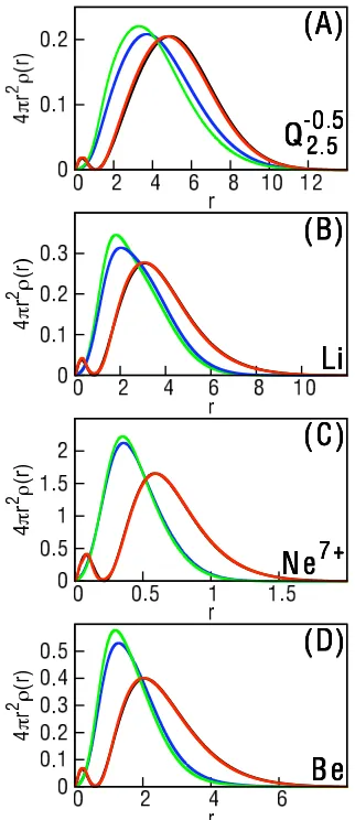
Figure 1.2: The 2s electron density (ρA) for (A) the Q2−.50.5 ion, (B) the Li atom,

(C) the Ne+7 ion, and(D) the Be atom. Calculations performed using e-DFT with the non-additive kinetic energy calculated using our exact protocol (red), the TF functional (blue), and the TFvW functional (green). The black curve, which is nearly indistinguishable from the exact protocol, presents the results from the full KS-DFT calculation.

(32)

as well as the four-electron Be atom. For each application, ρA was chosen to include

a single 2s electron, and the remaining electrons were included in ρB. In addition

to using the exact embedding protocol described here, the NAKP in the embedding

calculations was treated using the approximate TF kinetic energy functional (TTF[ρ] ,

Eq. 1.13) and the TFvW functional with the standard 1/9 mixing parameter (TTF[ρ]+

1

9TvW[ρ]).

Fig. 1.2 presents the ρA obtained in these e-DFT calculations. For reference,

Fig. 1.2 also includes the 2s orbital density from the full KS-DFT calculation.

Ab-solute agreement between the KS-DFT results and the e-DFT results would only

be expected if all results were obtained with the exact exchange-correlation

func-tional. Nonetheless, since all calculations in this study employ the same approximate

exchange-correlation functional, comparison of the e-DFT and KS-DFT results

pro-vides a significant test of the accuracy of the various NAKP descriptions.

Fig. 1.2 clearly demonstrates the sensitivity of e-DFT calculations to the method

of treating the NAKP. In comparison to KS-DFT, the e-DFT results from the

approx-imate TF and TFvW functionals are peaked at significantly shorter radial distances,

and they qualitatively fail to capture the nodal structure. Interestingly, the vW

correction to the TF functional actually worsens the agreement with the KS-DFT

reference. The exact embedding protocol describe here, however, is graphically

indis-tinguishable from the KS-DFT result.

Further evaluation of the e-DFT methods can be obtained by comparing the

cal-culated one-electron ionization energies (IEs) for the various methods. The e-DFT

IE is calculated from the difference between the total electron energy from Eq. 3.6

and the energy from a full KS-DFT calculation performed on the ionized (N-1

elec-tron) system. These results are presented in Table 1.1, which again illustrates the

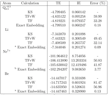
qualitative shortcomings of the approximate NAKP treatments. For the approximate

(33)

result for the IEs ranges from 30-60% for 3-electron systems, and up to 80% for Be.

As has been observed previously,40 including the vW gradient correction decreases the accuracy of the IE calculation. The exact embedding protocol almost completely

eliminates these differences with the reference calculation, with errors of less than

0.2% for Q−₂_.0₅.5, Li, and Be and with an error of less 4% for Ne7+.

The lower accuracy of our embedding protocol for the case of Ne7+ arises from the description of the nuclear cusp. The KSCED equations converged slowly for this

case, and the convergence threshold had to be raised to 10−5 hartrees. By changing from GTOs to Slater-type orbitals (results not shown), the convergence problem was

removed, and it was found that for all four applications, the IEs obtained using our

e-DFT protocol were within 1% of the full KS-DFT result. Below, we describe how

the use of a simple switching function for the NAKP in the cusp region also removes

these convergence problems for the GTOs, while preserving the accuracy of the IE

calculation.

We note that the ionization of the closed shell Be atom presents an electronic

structure challenge that is similar to the homolytic cleavage of a covalent bond. From

the perspective of the NAKP, this atomic system is especially challenging since both

electrons in the 2s “bond” are co-localized on a single attractive center. The difficulty

of this particular case is confirmed by the especially poor description provided by the

TF and TFvW functionals for the IE of the Be atom. The excellent accuracy of the

new embedding protocol for this case suggests that the method will allow for accurate

e-DFT calculations in which the subsystems are linked by covalent bonds.

Fig. 1.3 illustrates the KSCED potentials, V_effKSCED[ρA, ρB;r], and the

correspond-ing NAKPs,vnad[ρA, ρB;r], that are obtained from the exact embedding calculations.

For each system, the similarity between these two potentials illustrates the

domi-nance of the NAKP at short distances. However, the NAKP decays rapidly, and the

(34)

[image:34.612.147.502.246.558.2]

Table 1.1: Total energy (TE) and ionization energy (IE) obtained using KS-DFT and e-DFT.

Atom Calculation TE IE Error (%)

Q−₂_.0₅.5

KS -4.799405 0.060142

-TFvW -4.835122 0.095258 59.99

TF -4.819221 0.079357 33.28

Exact Embedding -4.799510 0.060247 0.18 Li

KS -7.343870 0.201098

-TFvW -7.443321 0.300549 49.45

TF -7.408509 0.265737 32.14

a

Exact Embedding -7.344046 0.201274 0.09 Ne7+

KS -101.964612 8.754056

-TFvW -106.413890 13.203334 50.83

TF -105.630042 12.419486 41.87

b

Exact Embedding -102.294207 9.083650 3.77 Be

KS -14.447017 0.331698

-TFvW -14.717243 0.601924 81.47

TF -14.635950 0.520631 56.96

a _{Exact Embedding} _-14.447463 _0.328900 _0.13

a _{KSCED equations converged to 10}−7 _Hartree

(35)

Although it is not visible from the scale of the plots in Fig. 1.3, the vnad[ρA, ρB;r]

term comprises less than 1% of theV_effKSCED[ρA, ρB;r] for distances greater than 3 a.u.

[image:35.612.202.444.149.434.2]

for all cases. (For Ne7+, this regime is reached at 0.43 a.u.)

Figure 1.3: The KSCED effective potential, V_effKSCED[ρA, ρB;r], for (A) the Q−2.05.5

ion, (B) the Li atom, (C) the Ne+7 ion, and (D) the Be atom and the NAKP,

vnad[ρA, ρB;r], for (E) the Q2−.05.5 ion, (F) the Li atom, (G) the Ne

+7 _{ion, and} _(H)

the Be atom using the e-DFT protocol presented here.

Comparison of the NAKPs in Fig. 1.3E-H with the densities in Fig. 1.2 illustrates

that the nodal structure in the 2s electron density is enforced by the NAKP. For each

system, the large outer peak in the NAKP coincides with the nodal feature in the

2s density. Unlike the KS-DFT results, we note that the densities obtained using

e-DFT in Fig. 1.2 do not exhibit a genuine radial node, since ρA corresponds to the

ground-state eigenvector of Eq. 1.1. A large peak in the e-DFT effective potential

is therefore essential to achieve the correct 2s shell structure. The NAKPs obtained

(36)

(not shown), which leads to the poor descriptions for the 2s electron density (Fig.

1.2) and the IE (Table 1.1).

In addition to the pronounced outer-most peak for each NAKP in Fig. 1.3E-H,

oscillations at short distances are observed. This oscillatory behavior is sensitive to

the basis set representation. Small changes in the orbital coefficients for regions of low

density give rise to large changes in the kinetic potential (Eq. 1.24), resulting in slow

convergence of the KSCED equations. (These oscillations are not observed when the

density vanishes at large distances since the basis set expansion is dominated by only

the slowest-decaying function in that regime.) Using STOs rather than GTOs, the

NAKP oscillations at short distances were diminished (not shown), and the iterative

convergence was improved. In future applications of the exact embedding protocol

with GTOs, the use of the convergence acceleration algorithms such as DIIS39 may prove beneficial. However, we now demonstrate that the problems associated with

poor convergence and NAKP oscillations can be alleviated with a simple modification

of Eq. 1.24.

As ρAvanishes close to the nucleus, evaluation of the second term in Eq. 1.24

be-comes unstable, leading to the aforementioned convergence problems. This is avoided

by introducing a switching function that changes from the exact expression for the

kinetic potential of subsystem A to the corresponding TF approximation near the

nucleus,

vnad[ρA, ρB;r] =

2

ρAB(r)

NAB/2

X i=1 −1 2φ AB

i (r)∇2φABi (r)−iφABi (r)2

(1.25)

− 2

ρA(r)

NA/2

X i=1 −1 2φ A

i (r)∇2φAi (r)−Ai φAi (r)2

× (1.26)

(1−f[ρB;r])−

5 3CTF ρ

2/3 A

(37)

where f[ρB;r] is the smooth switching function

f[ρB;r] =

1

eκ(−ρB(r)+ρ0B)+ 1

. (1.27)

Previous work used a similar function to switch between approximate expressions for

the NAKP in the vicinity of the nuclear cusp.40 The parameters ρ0_B and κ determine the radial distance and the abruptness with which switching occurs, respectively. The

parameterρ0_Bwas related to the integrated electron density in the cusp region, setting

ρ0_B =ρB(r0), where

ξ = 4π Z r0

0

r2ρB(r)dr. (1.28)

e-DFT results obtained using range of values for κand ξ were compared to deter-mine robust parameters for the switching function. Setting κ = 50, we varied ξ over the range from 0.4 to 0.8 for Li and Ne7+, which led to changes in the total calculated energy of less than 0.4 mH and 5 mH, respectively. Similarly, setting ξ = 0.6 and

varying κ over the range from 50 to 500 led to differences of less than 0.1 mH for both Li and Ne.

Using the NAKP expression in Eq. 1.27 with ξ= 0.6 andκ= 50, our e-DFT pro-tocol was applied to all four systems, and the results are presented in Table 1.2. All

calculations reached full 10−8 convergence within 80 iterations of the KSCED equa-tions, in contrast with the calculations using Eq. 1.24, which was difficult to converge

in some cases even with 2000 iterations. Furthermore, the e-DFT calculations with

the modified NAKP expression in Eq. 1.27 yields excellent accuracy in comparison

to the full KS-DFT equations, with less than 1.5% error in the IE for all cases.

For the Li atom, Fig. 1.4 compares the NAKP, the KSCED effective potential,

and the 2s electron density obtained by solving the KSCED equations using either

Eq. 1.24 (black) or Eq. 1.27 (red) for the NAKP. The black curves in this figure are

(38)

[image:38.612.205.443.110.186.2]

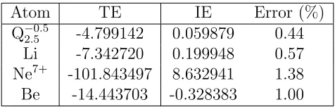
Table 1.2: Total energy (TE) and ionization energy (IE) obtained using e-DFT with the NAKP switching function (Eq. 1.27).

Atom TE IE Error (%)

Q−₂_.0₅.5 -4.799142 0.059879 0.44 Li -7.342720 0.199948 0.57 Ne7+ -101.843497 8.632941 1.38 Be -14.443703 -0.328383 1.00

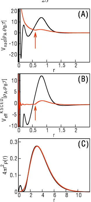
distances, the switching function produces a relatively featureless, repulsive NAKP

due to the TF approximation; the arrow in this figure indicates the radial distancer0

that corresponds to the parameter ξ = 0.6. Fig. 1.4B illustrates that the repulsive NAKP largely cancels the attractive electron-nuclear Coulomb term in the KSCED

effective potential (Eq. 1.5). As ρA vanishes at the nucleus, the KSCED effective

potential must also approach zero.30 The remaining oscillations at radial distances in Fig. 1.4B are an artifact of the finite basis set. Finally, Fig. 1.4C demonstrates

that the 2s electron density that is obtained using the switching function does not

reproduce the features of the radial node, but it recovers the exact embedding result

for distances beyond 1 a.u. This close agreement at large distances is expected41 from the accuracy of the IE calculations in Table 1.2. In light of the much improved

convergence efficiency, use of the NAKP expression in Eq. 1.27 compares favorably

with exact embedding via Eq. 1.24.

1.5 Extension to Larger Systems

The calculations reported here demonstrate a proof-of-principle for the exact

calcula-tion of the NAKP. However, for applicacalcula-tions of e-DFT to large systems, performance

of the ZMP extrapolation at each iteration of the KSCED equations is impractical.

Nonetheless, the short-ranged nature of the NAKP (see Fig. 1.3E-H) suggests several

strategies for employing our e-DFT protocol in larger systems.

(39)

[image:39.612.247.403.59.403.2]

Figure 1.4: (A) The NAKP, (B) the KSCED effective potential, and (C) the 2s electron density (ρA) for the Li atom, obtained using exact embedding (black) and

using the modified NAKP in Eq. 1.27 (red). The arrow indicates the radial distance at which switching occurs.

. . ., Bf), and consider the sum of the NAKP terms due to the individual fragments,

vnad[ρA, ρB;r]≈

f X

i=1

δTs[ρ]

δρ

ρ=ρA+ρ_Bi

− δTs[ρ] δρ

ρ=ρA

. (1.29)

This equation is exact in the limit of one fragment, and its implementation with our

protocol will avoid ZMP extrapolation for anything larger than the union of subsystem

A with a single fragment.

The assumption in Eq. 1.29 that the NAKP is additive among the fragments

(40)

corrected using the TF (or other) approximate kinetic energy functional,

vnad[ρA, ρB;r] ≈

δTs[ρ]

δρ

(appr)

ρ=ρA+ρB

− δTs[ρ] δρ

(appr)

ρ=ρA

!

− f X

i=1

δTs[ρ]

δρ

(appr)

ρ=ρA+ρ_Bi

− δTs[ρ] δρ

(appr)

ρ=ρA

!

+

f X

i=1

δTs[ρ]

δρ

(exact)

ρ=ρA+ρ_Bi

− δTs[ρ] δρ

(exact)

ρ=ρA

!

. (1.30)

Here, the first term on the RHS corresponds to the NAKP obtained from the TF

functional for the full system. In the second term, the contribution due to each of the

fragments using the TF approximation is removed, and in the third term, each of the

fragment contributions is replaced using the exact protocol. The short-ranged nature

of the NAKP suggests that distance-based cutoffs can be employed with summations

in Eqs. 1.29 and 1.30, allowing for significant computational savings.

1.6 Conclusions

We have described a general and exact protocol for treating the non-additive kinetic

potential in embedded density functional theory calculations. In applications to a

series of three- and four-electron systems, we have numerically demonstrated the

ap-proach, and we have illustrated the qualitative failures that can arise from the use

of approximate kinetic energy functionals. We have also shown that improved

con-vergence of the KSCED equations can be obtained with appropriate switching of the

NAKP in the vicinity of the nuclear cusps, and we have described possible strategies

for the scalable implementation of our embedding protocol in large systems.

Natu-ral applications of exact embedding include the rigorous calculation of one-electron

pseudopotentials, the calculation of DFT embedding potentials for use with high-level

(41)

of the “molecular embedding” strategy in which each molecule of a large system is

assigned to a different embedded subsystem.44

1.7 Appendix: Unrestricted Open-Shell e-DFT

For unrestricted open-shell e-DFT calculations, the density of each subsystem is

fur-ther partitioned intoα andβ spin densities, such thatρAB=ραA+ρ

β

A+ρ

α

B+ρ

β

B. This

leads to the KSCED equations

−1

2∇

2₊_VKSCED eff [ρ

α

A, ρ

β

A, ρ

α

B, ρ

β

B;r]

φA,α_i (r) = A,α_i φ_iA,α(r) i = 1, ..., N_Aα, (1.31)

−1

2∇

2₊_VKSCED eff [ρ

β

A, ρ

α

A, ρ

β

B, ρ

α

B;r]

φA,β_i (r) = A,β_i φ_iA,β(r) i = 1, ..., N_Aβ, (1.32)

−1

2∇

2₊_VKSCED eff [ρ

α

B, ρ

β

B, ρ

α

A, ρ

β

A;r]

φB,α_i (r) =B,α_i φ_iB,α(r) i = 1, ..., N_Bα, (1.33)

−1

2∇

2₊_VKSCED eff [ρ

β

B, ρ

α

B, ρ

β

A, ρ

α

A;r]

φB,β_i (r) =B,β_i φ_iB,β(r) i = 1, ..., N_Bβ. (1.34)

Here, N_µν is the number of electrons in each subsystem, and ρν_µ(r) =

Nν µ X

i=1

|φµ,ν_i (r)|2_,

whereµ∈ {A,B}andν ∈ {α, β}. The KSCED effective potential,V_effKSCED[ρα_A, ρβ_A, ρα_B, ρβ_B;r], is

V_effKSCED[ρα_A, ρβ_A, ρα_B, ρβ_B;r] =vne(r)+vJ[ρAB;r]+vxc[(ραA+ρ

α

B),(ρ

β

A+ρ

β

B);r]+vnad[ραA, ρ

α

B;r]

(1.35)

where vne(r) and vJ[ρAB;r] are unchanged from Eq. 1.5, vxc[(ραA+ρ

α

B),(ρ

β

A+ρ

β

B);r]

is the usual open-shell exchange-correlation potential for the total system,8 and the NAKP is discussed below.

The kinetic energy functional is separable into two different spin contributions8

Ts[ραµ, ρ β

(42)

where

Ts[ραµ,0] = Nα

µ X

i=1

hφµ,α_i | − 1

2∇

2_|φµ,α

i i (1.37)

and likewise for Ts[0, ρβ]. Therefore, the NAKP depends only on spin densities

cor-responding to the same spin, such that

vnad[ραA, ρ

α

B;r] =

δTs[ρα,0]

δρα

ρα₌_ρα

A+ραB

(r)− δTs[ρ α_,_0] δρα

ρα₌_ρα

A

(r), and (1.38)

vnad[ρβA, ρ

β

B;r] =

δTs[0, ρβ]

δρβ

ρβ₌_ρβ

A+ρ

β

B

(r)− δTs[0, ρ β_]

δρβ

ρβ₌_ρβ

A

(r). (1.39)

The ZMP extrapolation is used to calculate the KS spin orbitals {φAB_i ,ν} and eigenvalues{AB_i ,ν}for the full system, exactly as is described in the text, except that the total spin density is employed instead of the total electron density. Finally, our

exact expression for the NAKP for open-shell systems is modified from Eq. 1.24 as

follows:

vnad[ρνA, ρ

ν

B;r] =

1

ρν

AB(r)

N_Aν+N_Bν X i −1 2φ AB,ν i (r)∇

2_φAB,ν

i (r)−

AB,ν

i φ

AB,ν i (r)

2

− 1

ρν

A(r)

Nν A X i −1 2φ A,ν i (r)∇

2

φA,ν_i (r)−A,ν_i φA,ν_i (r)2

. (1.40)

The TF approximation for the non-additive kinetic energy in an open-shell

calcu-lation is

T_TFnad[ρν_A, ρν_B] = 22/3CTF

Z

ρν_AB5/3(r)−ρν_A5/3(r)−ρν_B5/3(r)dr, (1.41)

and corresponding result for the TFvW functional is

T_TFvWnad [ρν_A, ρν_B] =T_TFnad[ρν_A, ρν_B] + 1 72

Z |∇ρν

AB(r)|2

ρν

AB(r)

− |∇ρ ν

A(r)|2

ρν

A(r)

−|∇ρ ν

B(r)|2

ρν

B(r)

dr.

(43)

Bibliography

[1] P. Cortona, Phys. Rev. B44, 8454 (1991).

[2] T. A. Wesolowski and A. Warshel, J. Phys. Chem. 97, 8050 (1993).

[3] N. Govind, Y. A. Yang, A. J. R. da Silva, and E. A. Carter, Chem. Phys. Lett.

295, 129 (1998).

[4] T. A. Wesolowski,Computational Chemistry: Reviews of Current Trends, edited

by J. Leszczynski (World Scientific, Singapore, 2006), Vol. 10, 1-82.

[5] T. Kl¨uner, N. Govind, Y. A. Yang, and E. A. Carter, J. Chem. Phys. 116, 42 (2001).

[6] G. Hong, M. Strajbl, T. A. Wesolowski, and A. Warshel, J. Comp. Chem. 21, 234110 (2000).

[7] M. Hodak, W. Lu, and J. Bernholc, J. Chem. Phys. 128, 014101 (2008). [8] R. G. Parr and W. Yang, Density-Functional Theory of Atoms and Molecules

(Oxford University Press, New York, 1989).

[9] A. W. G¨otz, S. M. Beyhan, and L. Visscher, J. Chem. Theory Comput.5, 3161 (2009).

[10] T. A. Wesolowski, J. Chem. Phys.106, 8516 (1997).

(44)

[12] V. V. Karasiev, S. B. Trickey, and F. E. Harris, J. Comput.-Aided Mater. Des.

13, 111 (2006).

[13] F. Tran and T. A. Wesolowski, Int. J. Quantum Chem. 89, 441 (2002). [14] C. R. Jacob and L. Visscher, J. Phys. Chem. 128, 155102 (2008).

[15] S. M. Beyhan, A. W. G¨otz, C. R. Jacob, and L. Visscher, J. Chem. Phys. 132, 044114 (2010).

[16] L. H. Thomas, Proc. Camb. Phil. Soc. 23, 542 (1927). [17] E. Fermi, Z. Phys. 48, 73 (1928).

[18] C. F. von Weizs¨acker, Z. Phys. 96, 431 (1935).

[19] J. P. Perdew, J. Chevary, S. Vosko, K. A. Jackson, M. R. Pederson, D. Singh,

and C. Fiolhais, Phys. Rev. B. 46, 6671 (1992). [20] A. D. Becke, J. Chem. Phys. 84, 8 (1986).

[21] Y. A. Wang, N. Govind, and E. A. Carter, Phys. Rev. B 60, 16350 (1999). [22] J. A. Alonso and L. A Girifalco, Phys. Rev. B17, 3735-3743 (1978).

[23] P. Garc´ıa-Gonz´alez, J. E. Alvarellos, and E. Chac´on, Phys. Rev. B53, 9509-9512 (1996).

[24] S. Fux, K. Kiewish, C. R. Jacob, J. Neugebauer, and M. Reiher, Chem. Phys.

Lett. 461, 353 (2008).

(45)

[28] Q. S. Zhao, R. C. Morrison, and R. G Parr, Phys. Rev. A 50, 2138 (1994). [29] R. A. King and N. C Handy, Phys. Chem. Chem. Phys. 2, 5049-5056 (2000). [30] C. R. Jacob, S. M. Beyhan, and L. Visscher, J. Chem. Phys.126, 234116 (2007). [31] O. Roncero, M. P. de Lara-Castells, P. Villarreal, F. Flores, J. Ortega, M.

Pani-agua, and A. Aguado, J. Chem. Phys. 129, 184104 (2008).

[32] O. Roncero, A. Zanchet, P. Villarreal, and A. Aguado, J. Chem. Phys. 131, 234110 (2009).

[33] P. Huang and E. A. Carter, J. Chem. Phys. 125, 084102 (2006). [34] T. H. Dunning, J. Chem. Phys. 90, 1007 (1989).

[35] J. C. Slater, Phys. Rev. 81, 385-390 (1951).

[36] S. H. Vosko, L. Wilk, and M. Nusair, Can. J. Phys.58, 1200-1211 (1980). [37] B. N. Papas and H. F. Schaefer, III, J. Mol. Struc.: THEOCHEM 768, 175

(2006).

[38] M. R. Pederson and K. A. Jackson, Phys. Rev. B 41, 7453 (1990). [39] P. Pulay, Chem. Phys. Lett.72, 393 (1980).

[40] J. M. L. Lastra, J. W. Kaminski, and T. A. Wesolowski, J. Chem. Phys. 129, 074107 (2008).

[41] D. J. Tozer and H. C. Handy, Molec. Phys. 101, 2669 (2003).

[42] P. Huang and E. A. Carter, Annu. Rev. Phys. Chem. 59, 261 (2008).

(46)

(47)

Chapter 2 Embedded density functional theory for covalently

bonded and strongly interacting subsystems

2.1 Introduction

Important methodological challenges in electronic structure theory include the

long-timescale simulation ofab initio molecular dynamics and the seamless combination of

high- and low-level electronic structure methods in complex systems. Methods that

exploit the intrinsic locality of molecular interactions have demonstrated encouraging

progress towards these goals.1–17

In particular, orbital-free embedded DFT (e-DFT) offers a formally exact

ap-proach to electronic structure theory in which the interactions between subsystems

are evaluated in terms of their electronic densities.1–4 Recent work has demonstrated that constructing the embedded subsystems from individual molecules leads to a

linear-scaling electronic structure approach that maps naturally onto

distributed-memory parallel computers,13,18 and it provides a systematic framework for calculat-ing electronic excited states in condensed phase systems.19,20 However, approximate treatments of the non-additive kinetic potential (NAKP) limit the accuracy of this

approach in applications involving strongly interacting subsystems.21 For example, severe artifacts in the structure of liquid water, including the complete absence of a

second peak in the oxygen-oxygen radial distribution function, have been predicted

(48)

co-valently bonded embedded subsystems have also been shown to qualitatively fail.21–23 The development of improved methods to address the NAKP problem will open new

doors for on-the-fly, massively parallel electronic structure calculations in general,

condensed-phase systems.

In this paper, we describe progress towards the development of accurate, scalable

treatments for the NAKP in e-DFT. We provide the first molecular applications of

our recently developed Exact Embedding (EE) method,24 demonstrating that it suc-cessfully describes the breaking of covalent bonds and hydrogen bonds with chemical

accuracy. Additionally, we introduce and numerically demonstrate a pairwise

ap-proximation to the NAKP, which allows for the scalable implementation of the EE

method in large systems. Benchmark calculations are presented for systems with up

to 125 molecules, demonstrating that parallel implementation of the method enables

constant system-size scaling of the wall-clock calculation time.

2.2 Theory

2.2.1 Orbital-Free Embedded DFT

We utilize the orbital-free e-DFT formulation of Cortona1and Wesolowski and cowork-ers.2,3 For the case in which the total electronic density ρAB is partitioned into two

subsystems, ρAB =ρA+ρB, the corresponding one-electron orbitals obey the

Kohn-Sham Equations with Constrained Electron Density (KSCED),3

−1

2∇

2₊_v

eff[ρA, ρAB;r]

φA_i (r) =A_i φA_i (r) (2.1)

−1

2∇

2

+veff[ρB, ρAB;r]

(49)

where i= 1, . . . , NA, j = 1, . . . , NB, and NA and NB are the number of electrons in the respective subsystems. veff is the effective potential for the coupled one-electron

equations, such that

veff[ρA, ρAB;r] = vne(r) +vJ[ρAB;r] +vxc[ρAB;r]

+ vnad[ρA, ρAB;r], (2.3)

where the Nnuc nuclei occupy positions {Ri},

vne(r) = −

Nnuc

X i

Zi |r−Ri|

, (2.4)

vJ[ρ;r] =

Z _ρ₍_r0₎ |r0 ₋_r_|dr

0

, (2.5)

vxc[ρ;r] =

δExc[ρ]

δρ

(r), (2.6)

and Exc[ρ] is the exchange-correlation functional. vnad[ρA, ρAB;r] is the potential due

to the non-additive kinetic energy for non-interacting electrons, such that

vnad[ρA, ρAB;r] =

δTnad

s [ρA, ρB]

δρA

(r), (2.7)

where T_snad[ρA, ρB] ≡ Ts[ρAB]−Ts[ρA]−Ts[ρB]. The subsystem densities are

con-structed from the corresponding KS orbitals, using ρA(r) =

NA X

i=1

|φA

i (r)|2 and ρB(r) =

NB

X j=1

|φB

j(r)|

2_{. Eqs. 3.1-2.7 are easily generalized for the e-DFT description of multiple}

embedded subsystems.1,18

Two aspects of e-DFT are worth emphasizing. Firstly, like conventional

Kohn-Sham (KS)-DFT, it is a theory that is exact in principle, but practical calculations

must employ approximations to the unknown exchange-correlation functional.

(50)

intro-duces the NAKP, vnad[ρA, ρAB;r], since the one-electron orbitals for subsystem A

are not necessarily orthogonal to those of subsystem B. Without knowledge of the

exact functional for the non-interacting kinetic energy, this creates a second source

of approximation in e-DFT calculations. The significance of the NAKP is

system-dependent, with the most severe cases including those for which the subsystem

den-sities greatly overlap; no approximate kinetic energy functional has been previously

demonstrated to yield accurate results for embedded subsystems that are connected

by covalent bonds.3,21,22,25,26

2.2.2 Exact Calculations of NAKP

We have recently developed the Exact Embedding (EE) method to calculate the

NAKP.24 The general method can be summarized for two embedded subsystems as follows: A Levy constrained search (LCS)27 or equivalent technique is first used to determine the full set of orthogonal KS orbitals, {φAB

i }, that correspond to the total

density ρAB from the latest iteration of Eqs. 3.1-2.3. Then, from the KS orbitals

{φAB

i },{φ

A

i }, and{φ

B

i}, the corresponding kinetic potentials are calculated using the

exact result of King and Handy,28

vTs(r) =

Pn i=1(−

1

2φi(r)∇ 2_φ

i(r))−iφi(r)2)

ρ(r) +µ, (2.8)

where n is the number of occupied orbitals, i is the KS eigenvalue corresponding to

orbital φi, and µ is a constant. Finally, the NAKP needed for the next iteration of

Eqs. 3.1-2.3 is calculated directly from the difference

vnad[ρA, ρAB;r] =vTABs (r)−v

A

(51)

where the superscripts in this equation indicate the orbital set to which each kinetic

potential corresponds.

Rather than explicitly performing the LCS, we use the equivalent protocol of Zhao,

Morrison, and Parr (ZMP)29–31to obtain the exact non-interacting kinetic energy and the KS orbitals {φAB_i }. This requires solution of the following one-electron equations

−1

2∇

2

+vext(r) +vcλ(r)

φAB_i,λ(r) =AB_i,λφAB_i,λ(r) (2.10)

in the limit λ→ ∞, wherei= 1, . . . ,(NA+NB), and

v_cλ(r) = λ Z

ρ(r0)−ρAB(r)

|r0₋_r_| dr 0

. (2.11)

vext(r) corresponds to any well-behaved external potential,30,31 and various choices

for this potential are described in Sec. III B. In practice, Eq. 2.10 is solved at several

large, finite values ofλ, and the KS orbitals and eigenvalues, as well as the final non-interacting kinetic energy, are obtained via extrapolation.29–31 In Sec. V, we discuss a technique to robustly implement the ZMP step for NAKP calculations in large

systems.

The EE method outlined in Eqs. 2.8 - 2.11 is unique in that it allows for the

for-mally exact calculation of the total electronic density within the e-DFT framework,

using integer orbital occupancies and without approximations to the NAKP. The

method was previously demonstrated for atomic systems with strongly overlapping

subsystem densities,24and the current paper presents its first molecular applications. We note that several other groups have also used density inversion techniques to

cal-culate the NAKP, assuming that the total electron density is already available from