User-Assisted Feature Correspondence Matching
Dan Ring, Anil Kokaram
[email protected], [email protected]
Sigmedia Group, School of Electronic & Electrical Engineering, Trinity College Dublin.
Abstract
Feature matching is a vital stage in many image processing applications. Finding accurate correspondences is made difficult by phenomena such as occlusions, non-rigid deformations, motion blur and more. We posit that some scenarios do not have enough information for an accurate automatic solution. Although many applications are required to be automatic, there are others that can benefit from being semi-automatic, allowing the user to provide assistance to areas where the system is failing. Good examples of this exist in the media post-production world, such as multi-view scene reconstruction, sparse-to-dense disparity estimation from view matching, image mosaic’ing (digital panoramas), or even motion estimation. The presented paper describes how to incorporate user-assistance into a Bayesian feature matching framework. By adding user information in the form of intuitive Bezier curves, difficult regions can be matched with the same accuracy as easier to match areas. The presented system uses a simple optimisation scheme, giving the user real-time interactive control over the corrected matches.
Keywords: Feature-Points, Feature Matching, User-Assisted, MRF, ICM
1 Introduction
Feature matching is an important part of many image processing tasks, such as image registration, object tracking, multi-view scene reconstruction and depth estimation from stereo image pairs. The accuracy of these higher level tasks depends on the accuracy of matching features. In real world images, feature matching is made difficult by non-rigid object motion, blurring and poor textural content (pathological content). There is often not enough information to automatically reject incorrect matches or propose better alternative matches. Given that user intervention is typical in post-production, we propose an interactive system to allow the user to encourage better feature matches in difficult regions, examples of which are shown in Figures 2 & 1.
[image:1.595.310.548.188.350.2]Given sets ofsparse features in two frames (such as Harris-Laplace corners [6, 5] or SIFT features [8]), previous work concentrates on finding correct correspondences between them. Most matching strategies compare local “descriptors”, around the sites of the features. A low descriptor distance between a pair of features indicates a likely match. Simple heuristics
Figure 2: Example of a registration task. Top: A transformation is estimated between the two images using RANSAC, and the best correspondences are shown (blue). The model did not capture the perspective distortion and missed possible matches on a number of buildings. Bottom: two simple curves are provided by the user as a rough guide (yellow), and the previously overlooked matches are recovered (green).
such as “nearest-neighbour” and “ratio-testing” [8] attempt to match based solely on descriptor distances, disregarding the spatial context of the features. It is sensible that incorporating spatial feature context in some way, can improve feature matching performance. For example, by estimating piece-wise transformations of subsets of features [13], or requiring that at leastN similar feature correspondences lie in the vicinity of a potential match [11].
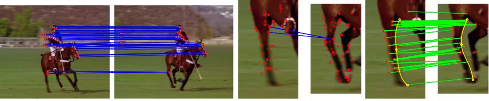
Figure 1:Some scenes do not have enough information to provide accurate feature matches. A selection of the strongest correspondences is given between the two frames in (left, blue), using the default matching scheme described in Section 3. Regardless of parameters, correspondences are never identified between the flat untextured regions of the horse, although features do indeed exist for these areas (centre, red). Following the manual addition of 2 Bezier curves to the shape of the horse’s leg in the right image (yellow), matches are encouraged and identified in the difficult regions (green).
is the field of object segmentation[4, 1].
Torresani et al. [14] pose the problem of matching using an energy that combines spatial information with descriptor matching. Graph matching techniques are then used to solve the resulting optimisation problem. Despite improved matching performance, problematic regions (withpathological content) remain difficult. Figure 1 shows an example of feature correspondences similar to those found by Torresani et al. between a pair of images in a sequence. There are no feature matches found on the horse’s legs due to a combination of heavy deformation and blur. However, visually it can be seen that matches should exist in these regions. Other related work that explicitly detects non-rigid deformation [10], or similarly performs quasi-dense matching [7], relies on first finding a small set of reliable matches. Again, the number of features matched in Figure 1 (centre pair) is insufficient as bootstrap matches. This reaffirms our premise that some situations simply do not have enough information to provide accurate feature correspondences.
The novelty in this paper is the development of a feature matching energy function that incorporates user information. The user is encouraged to draw two smooth curves roughly covering corresponding, yet unmatched regions. Feature matches are then encouraged in the vicinity of these curves. The advantage of this technique is that the algorithm is not restricted to the exact form of the curves, giving a good interface for user input. This provides an interactive method of correcting mistakes at the feature matching level. The new matching framework is presented next, and the process of user interaction is described. Results are discussed in Section 3.
2 User-Assisted Matching Framework
Following [14], consider that P0 and P00 are the features detected in two images, and A ⊆ P0 ×P00 denotes the set of possible assignments between these features. Amatching configuration is defined by the binary-valued vector x ∈ {0,1}A. A potential correspondencea ∈ Aindexes an entry
xain the vectorx. The correspondenceaexists ifxa= 1, and
does not exist ifxa= 0. Given a featurep∈P0,A(p)is the set
of correspondences inP00involvingp. The objective is to find a matching configurationxthat minimises an energy function as follows.
E(x) =λappEapp(x) +λusrEusr(x) +λgeoEgeo(x) (1) The components of E(x)are the feature appearance energy, Eapp(x), our proposed user-assisted energy,Eusr(x), and the spatial consistency energy,Egeo(x), each of which is described below. The scalarsλapp,λusrandλgeoweight the contribution of the respective energy terms.
Feature Appearance, Eapp(x): The function Eapp(x)
measures the dissimilarity between a pair of features by comparing the pixel neighbourhoods around the feature sites. The image regions around the sites are described by SIFT descriptors [8] to allow for high amounts of geometric variation, such as non-rigid deformations.Eapp(x)is therefore
given by:
Eapp(x) = X
a∈A(p)
xakd(I0,p)−d(I00,q)k
whered(I0,p)andd(I00,q)are the SIFT descriptors calculated
about sitespandqof featurespandq∈A(p).
User Assistance, Eusr(x): In this energy, cubic
user-defined Bezier curves encourage correspondences in difficult to match regions. Bezier curves are already used in most image and video editing and compositing tools, making them a natural choice for user input in this situation. Imagine a region corresponding between two images exists, but is unable to be matched. In this case, the user marks the region in both images with a rough Bezier curve, an example is shown in Figure 1 (right). The cubic Bezier curve equation parameterised byt∈ {0,1}is given as follows:
B(t) = (1−t)3P0+ 3(1−t)2tP1+ 3(1−t)t2P2+t3P3
whereP0,P1,P2, andP3are 2D control points in the image
Intuitively, we want to use the curves as a transform function, taking locations of features around the curve in image one, and projecting them onto corresponding locations about the second curve in image two. It is not expected that the projected feature locations will match exactly to features in the second image, but the idea is to use the transformation as a soft constraint to encourage matches in the vicinity of the projected locations.
Imagine two curves B1(t) and B2(t) belonging to images
one and two respectively. For a location p, the value of the curve parameter t giving the lowest distance between p and the curve B1(t) is found, and used to calculate the
corresponding location on the second curve,B2(t). Using the
local gradients of the curves, the vector angle and distances between the original and projected points are preserved. This curve transform functionfis defined as follows:
f(p) =B2(n(B1,p)) +ρ
cos(θ) sin(θ)
−sin(θ) cos(θ)
n(B,p) = arg min
t
kB(t)−pk
where:
ρ=kB1(n(B1,p))−pk
θ= ∠n(p−B1(n(B1,p))−dB1dt(t)|t=n(B1,p)
o
+ ∠ndB2(t)
dt |t=n(B1,p)−
dB1(t)
dt |t=n(B1,p)
o
The functionn(B,p)finds the parametertof the curve closest to the locationp. The numeric solution to this can be found in Graphic Gems [9]. We now have to incorporate the function f into an energy function. Given two features pandq from images one and two respectively, we propose the function Eusr(x)that encourages matches where the projected location f(p)and feature locationqare low:
Eusr(x) = X
a∈A(p)
xa
kf(p)−qk2
r2
wherer is a scalar to weight the disparity betweenf(p)and q. To limit the influence of the curves to the difficult regions, the variableris set to some distance. The value ofrdepends on how tightly we want to constrain the projected sites about the transformationf, and will vary depending on the matching difficulty of the region. By limiting the transformation to a specific area, it is possible to add multiple curves, enabling the correction of multiple difficult regions in the same image.
Encouraging Spatial Smoothness,Egeo(x): Given a match
betweenpandq, we expect features in the neighbourhood of p(ps) to match to features in the neighbourhood ofq, (qs). The work by Berg et al. [2] from shape-matching literature describes a global geometric agreement of deformations between a set of feature matches. We adapt this idea into our energy functionEgeo(x)as follows.
Egeo(x) = X (a,b)∈N
xaxbη(eδ
2
a.b/σ
2
l−1)+(1−η)(eα
2
a,b/σ
2
α−1)
where:
δ(p,ps),(q,qs)=
|kp−qk − kps−qsk|
kp−qk+kps−qsk
α(p,ps),(q,qs)= arccos
p−q
kp−qk·
ps−qs kps−qsk
The functions δ(p,ps),(q,qs) and α(p,ps),(q,qs) measure the disagreement between the distances and directions of neighbouring translational vectors respectively, with the variableη ∈ {0,1} used to weight importance between the two. For this paper, we keep the variablesη,σl2,σα2 fixed at
0.5,4and4respectively.
The set of neighbouring feature matchesNis given by:
N={h(p, q),(ps, qs)i ∈A×A|
p∈Nps∨q∈Nqs∨ps∈Np∨qs∈Nq}
For example, given a match between featuresp∈ P0 andq∈ P00,ps ∈ P0 is in the neighbourhoodN
p ofp, and qs ∈ P00
is in the neighbourhoodNq ofq. A featurepsis considered to
be within the neighbourhoodNp if it is within the previously
defined distancer.
2.1 Energy Minimisation
Torresani et al. [14] use graph matching in order to find the optimal configuration for x. However, the advantage of a globally optimum solution comes at the expense of relatively long processing times. To allow a more interactive experience, where the user is presented with updated results following the addition or modification of a Bezier curve, we can make some observations that allow the fast but sub-optimal ICM [3] scheme to perform well.
Firstly, we note thatEapp(x)andEusr(x), do not depend on
neighbouring feature energies, and so need only be computed once. However,Egeo(x)is dependent on neighbouring feature
correspondences. The number of possible feature matches to be evaluated can be reduced by considering only those within the radiusrof the projection ofp,f(p). This set of candidates is defined asNr(p)⊆A(p).
At the beginning of the minimisation, we pre-calculate Eapp(ˆx)andEusr(ˆx), create a proposed match configuration ˆ
x, and randomly assign each featurepto a candidate feature inNr(p). At each iteration of ICM,Egeo(ˆx)is evaluated and
used to yieldE(xˆ)from Equation 1. For each featurep,xˆis then updated to select the entry inNr(p)with the minimum
corresponding energy inE(ˆx). The algorithm terminates when there are no further changes toˆxor at most 10 iterations have passed. The estimated configuration is given byˆx.
3 Results & Discussion
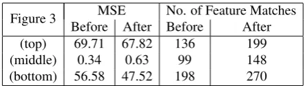
Figure 3 MSE No. of Feature Matches Before After Before After
(top) 69.71 67.82 136 199
(middle) 0.34 0.63 99 148
[image:4.595.58.280.70.133.2](bottom) 56.58 47.52 198 270
Table 1: Matching results before and after user interaction.
models of 3D objects given a large amount of views (8 in this case), and the correspondences between pairs can then be generated from the estimated 3D meshes. The MSE between our estimated feature matches and the ground truth set then gives a measure of the match quality.
For the non-user defined matching (Method N), correspondences are found by nearest-neighbour matching of SIFT descriptors of the features. Using the spatial consistency constraint of [11], a match (p, q) also requires at least k similar matches in the neighbourhoods Np and Nq, for our
experiments, we set k = 3, and the neighbourhood radius r= 15. Matches are also rejected if the descriptor differences are above a threshold, which we set at0.5. Good values of λapp,λusrandλgeofor Equation 1 were found experimentally to be0.707,5and5respectively. Results before and after user interaction are presented in Table 1, and shown visually in Figures 3.
It is encouraging that the MSE over all the features (user and automatic) does not change much from the MSE over the auto feature matching alone. In Figures 3, (top) & (bottom), the high degree of ambiguity in matching due to blur causes a higher MSE, while in Figure 3 (middle) the highly textured regions serve to lower the MSE. In both cases, the image conditions affect user and automatic features alike. In general then, the user generated feature matches are as good as the automatic ones, and the algorithm successfully incorporates this new information. Additional examples of user-assisted matching are shown in Figures 4, 5 and 6.
The results show that the algorithm is successful at increasing dramatically the number of useful matches with minimal intervention. Our future work explores the impact these new matches can have on the performance of various cinema post-production applications e.g. tracking and object segmentation.
References
[1] Xue Bai and Guillermo Sapiro. A geodesic framework for fast interactive image and video segmentation and matting. In Computer Vision, 2007. ICCV 2007. IEEE 11th International Conference on, pages 1–8, 2007.
[2] Alexander C. Berg, Tamara L. Berg, and Jitendra Malik. Shape matching and object recognition using low distortion correspondences. InCVPR, pages 26–33, Washington, DC, USA, 2005. IEEE Computer Society.
[3] J. Besag. On the statistical analysis of dirty pictures.
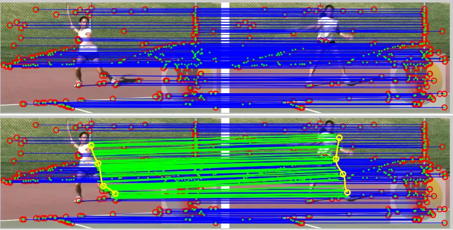
Figure 3: Scenes from a multi-view camera set-up. The pairs of images on the left show a sample of the strongest correspondences (blue) between the images using the scheme N. Matches are generally not found on the flat texture-less regions of the the legs are arms. In the images on the right, the user supplies corresponding Bezier curves (yellow) along the lines of limbs without matches, e.g. left leg (top-right), and left arms (middle- and bottom-right). Results of our guided matching are then shown in green on the right.
Journal of the Royal Statistical Society, Series B, 48:259– 302, 1986.
[4] Antonio Criminisi, Toby Sharp, and Andrew Blake. Geos: Geodesic image segmentation. InECCV (1), pages 99– 112, 2008.
[5] C. Harris and M. Stephens. A combined corner and edge detector. In4th Alvey Vision Conference, pages 147 – 151, 1988.
Figure 4: This example is interesting, although there are many correct matches in the scene, there are hardly any matches for the tennis player (top, blue). This is probably due to the non-rigid deformation and motion blur exhibited by the athlete. Drawing a simple set of roughly placed curves instantly generates reasonable matches for the marked side of the player. Note that the content between the frames has changed (for example, the players left leg has turned inwards), and so how useful the new features are depends largely on the target system.
Figure 5: In this example severe interlacing artefacts make it very difficult to detect features. Notice that many of the originally matched features are actually incorrect (top, blue). After marking the head of the subject with a pair of curves, the algorithm has sufficient information to perform better matching.
[image:5.595.45.292.436.626.2][7] Maxime Lhuillier and Long Quan. Match propogation for image-based modeling and rendering. IEEE Trans. Pattern Anal. Mach. Intell., 24(8):1140–1146, 2002.
[8] David G. Lowe. Distinctive image features from scale-invariant keypoints. International Journal of Computer Vision, 60(2):91–110, November 2004.
[9] Philip J. Schneider. An algorithm for automatically fitting digitized curves. pages 612–626, 1990.
[10] I. Simon and S.M. Seitz. A probabilistic model for object recognition, segmentation, and non-rigid correspondence. In Computer Vision and Pattern Recognition, 2007. CVPR ’07. IEEE Conference on, pages 1–7, June 2007.
[11] J. Sivic and A. Zisserman. Video Google: Efficient visual search of videos. In J. Ponce, M. Hebert, C. Schmid, and A. Zisserman, editors,Toward Category-Level Object Recognition, volume 4170 of LNCS, pages 127–144. Springer, 2006.
[12] J. Starck and A. Hilton. Surface capture for performance based animation. IEEE Computer Graphics and Applications, 27:21–31, 2007.
[13] P. H. S. Torr. Geometric motion segmentation and model selection. Phil. Trans. Royal Society of London A, 356:1321–1340, 1998.