A method to employ the spatial organization of catchments into semi distributed rainfall–runoff models

https://doi.org/10.5194/hess-21-4259-2017 © Author(s) 2017. This work is distributed under the Creative Commons Attribution 3.0 License.

A method to employ the spatial organization of catchments into

semi-distributed rainfall–runoff models

Henning Oppel and Andreas Schumann

Institute of Hydrology, Water Resources Management and Environmental Engineering, Ruhr-University Bochum, Bochum, 44801, Germany

Correspondence to:Henning Oppel ([email protected]) Received: 11 April 2017 – Discussion started: 2 May 2017

Revised: 18 July 2017 – Accepted: 19 July 2017 – Published: 30 August 2017

Abstract. A distributed or semi-distributed determinis-tic hydrological model should consider the hydrologically most relevant catchment characteristics. These are heteroge-neously distributed within a watershed but often interrelated and subject to a certain spatial organization which results in archetypes of combined characteristics. In order to reproduce the natural rainfall–runoff response the reduction of variance of catchment properties as well as the incorporation of the spatial organization of the catchment are desirable. In this study the width-function approach is utilized as a basic char-acteristic to analyse the succession of catchment characteris-tics. By applying this technique we were able to assess the context of catchment properties like soil or topology along the streamflow length and the network geomorphology, giv-ing indications of the spatial organization of a catchment. Moreover, this information and this technique have been im-plemented in an algorithm for automated sub-basin ascer-tainment, which included the definition of zones within the newly defined basins. The objective was to provide sub-basins that were less heterogeneous than common separation schemes. The algorithm was applied to two parameters char-acterizing the topology and soil of four mid-European water-sheds. Resulting partitions indicated a wide range of applica-bility for the method and the algorithm. Additionally, the in-tersection of derived zones for different catchment character-istics could give insights into sub-basin similarities. Finally, a HBV96 case study demonstrated the potential benefits of modelling with the new subdivision technique.

1 Introduction

Hydrological models are instruments for structuring the knowledge of hydrological processes in their dependence on watershed characteristics. For the set-up of these models sev-eral initial decisions have to be made, e.g. the following.

– Which type of model has to be used?

– Which temporal resolution could be appropriate? – Which spatial resolution of the model would be

neces-sary and useful?

– Which way could the model be parameterized? It is obvious that all of these options will affect the effort of the model and all choices have to consider the modelling pur-pose. Furthermore, these choices are interrelated; for exam-ple, predominant soil properties define the dominant runoff process and should, hence, define the used model. Therefore, conceptual models of a natural watershed require its subdi-vision into spatial units which should be as homogeneous as possible. Hydrological modelling is the attempt to specify hydrological processes quantitatively under consideration of boundary conditions. These boundary conditions are mainly determined by spatially heterogeneously distributed catch-ment characteristics. There are several approaches to address this heterogeneity in models to enable work with more or less homogeneous units.

data, though the correct criteria would be the spatial hetero-geneity of hydrological characteristics within the river basin. If the heterogeneity is at a low level, neighbouring basins could be modelled in accordance. In the reverse case, i.e. at a high level of heterogeneity, sub-basins should be modelled separately with an especially adapted model taking into ac-count their specific characteristics (e.g. an urban watershed model). Subsequently each sub-basin needs to be treated as a unique modelling instance that should provide a minimum level of heterogeneity (regarding key catchment characteris-tics). This way each sub-basin would end up with its own unique model and/or parameter set to adjust the model to mimic its natural response.

Another option to address spatial heterogeneity within a watershed could be to split the catchment into so-called hy-drologic response units (HRUs). A single unit merges areas, or cells, within a basin displaying similar characteristics in-dependent of their respective spatial allocation, i.e. each unit is a unique modelling instance. The HRU approach is based on the key assumption that the variation of the hydrological process dynamics within the HRU must be low relative to the dynamics in another HRU (Flügel, 1995). HRUs are devel-oped by intersecting different data layers of different phys-iographic criteria. The delineation of HRUs by combinations of these layers requires a categorization of its characteristics (soils, land-use and vegetation types, topography, and geol-ogy) to keep the number of HRUs at a manageable level, both the selection of criteria and their subdivision into classes at an acceptable degree of heterogeneity within the hydrolog-ical system. Subject to the chosen technique or purpose of HRUs, their models omit the actual spatial allocation (Lind-ström et al., 1997; Schumann et al., 2000) or define coherent units (Dunn and Lilly, 2001; Soulsby et al., 2006; Müller et al., 2009; Nobre et al., 2011; Gharari et al., 2011). However, some of these models try to transfer geological information (Müller et al., 2009; Soulsby et al., 2006) or topographical information (Nobre et al., 2011; Gharari et al., 2011) to hy-drological processes and assume homogeneous conditions of the remaining parameters.

A third option to address spatial heterogeneity in hydro-logical modelling is the utilization of a distributed catchment characteristic as a covariant metric supporting the spatial dis-tribution of a lumped state variable. An example of this ap-proach is the use of the topographic index in the well-known TOP model as a characteristic of the spatial variability of the soil water content (Beven et al., 1984).

Since GIS layers are widely available, there is an obvious trend to incorporate these data into the ascertainment of spa-tial units. Most approaches are based on topography (Band, 1986; Moore and Grayson, 1991; Vogt et al., 2003; Lai et al., 2016) and focus on the extraction of stream networks and the network connectivity, utilizing topology-driven mod-elling concepts (Beven and Kirkby, 1979; Rodríguez-Iturbe and Valdés, 1979). Particularly the development of the geo-morphologic instantaneous unit hydrograph (GIUH) as well

as its enhancements like the geomorphological dispersion (Rinaldo et al., 1991; Gupta and Mesa, 1988) require sophis-ticated stream network derivation and analysis. Methods in-troduced by Band (1986) or Verdin and Verdin (1999) were developed to generate data to meet this requirement. Further-more, Snell and Sivapalan (1994) applied the width function, introduced by Kirkby (1976), to model the geomorphic struc-ture of networks. Snell and Sivapalan (1994) were able to demonstrate that GIUHs based on the width function provide a better geomorphic dispersion than GUIHs derived from Horton laws (Robinson et al., 1995; D’Odorico and Rigon, 2003; Rigon et al., 2016). This has been a further step to in-corporate remote sensed data in describing the organization of catchments. While the above-described methods are based on gridded digital elevation models (DEMs), other methods try to identify streamlines derived from DEM shapes, pro-ducing contour lines (Moore and Grayson, 1991; Lai et al., 2016) that are subsequently used as modelling instances.

The following sections of this paper will present a combi-nation of different methods to address spatial heterogeneity of watershed characteristics, utilizing patterns resulting from the spatial organization of catchments. Sivapalan (2005) pointed out that the organization of a catchment has a fun-damental influence on the hydrological system. He defined the organization of a catchment as patterns of symmetry be-tween soil, topography, and the stream network. These pat-terns could unveil underlying mechanisms that induce dis-charge behaviour. Combining soil data with the flow path lengths at hillslopes in particular could provide a better un-derstanding of lateral flow distribution processes (Grayson and Blöschl, 2001).

In this study we will present a method to address these pat-terns by combining the width function (Kirkby, 1976; Mesa and Mifflin, 1986) with soil properties like pore volume and topographic characteristics like surface slope. Unlike tradi-tional methods for spatial pattern evaluation (like point-by-point or optimal logical alignment methods; Grayson and Blöschl, 2001) we retain the allocation of catchment prop-erties. This analysis revealed the organization of the water-shed and gave indications of spatial heterogeneity gradations which could be useful for the set-up of an appropriate model structure.

pro-posed subdivision scheme were compared to a common sub-division/modelling set-up.

The presentation has been split into four sections.

– Data, giving references to observations in some of the basins during the description of the methodological de-velopment.

– Methodological development, including observations, considerations, and techniques to assess spatial patterns of catchment characteristics and their spatial organiza-tion. In this section the sequence of the proposed algo-rithms will be presented which was utilized to incorpo-rate the spatial organizations into the model.

– Method analysis, i.e. checking their applicability and their limits.

– Method application, including the subdivision case study and modelling application.

2 Data

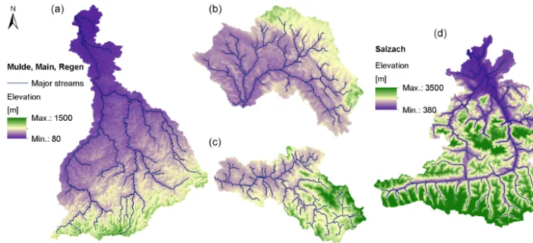
Due to the fact that the proposed methods were based on GIS-based catchment analysis, we first had to establish our database. In general, four catchments were selected to de-velop and test our methodological approach, with one catch-ment serving as a developcatch-ment catchcatch-ment and the remain-ing catchments for validation. Our development catchment was the Mulde River basin (Fig. 1, left). The basin is lo-cated mainly in eastern Germany, with a small section in the northern Czech Republic. Its southern section is located in the mid-range mountainous region of the Ore Mountains. With a size of 6170 km2it is the largest catchment used in this study. The other three catchments are the catchments of the rivers Regen (A=2613 km2, Fig. 1, lower middle), up-per Main (A=4224 km2, Fig. 1, upper middle), and Salzach (A=5995 km2, Fig. 1, right). While the Mulde, Main, and Regen basins are mid-mountainous catchments, the Salzach basin is an Alpine catchment. All catchments have different geomorphologic structures and river network types. While in the first three catchments, higher mountains are nearly exclusively located at the outer catchment boundaries, the Salzach catchment contains three high mountains located in the centre of the catchment. The two main tributaries encom-pass these mountains. While the Mulde River basin has a nearly continuous increase in slope and elevation from north to south, the topography of the remaining catchments is much more heterogeneous.

A DEM is essential for the proposed methods and the al-gorithm. We used a gridded DEM derived from the Shuttle Radar Topography Mission (SRTM) with a regular resolution of 100 m. By application of the D8 algorithm the required data, i.e. flow directions, flow length, and flow accumula-tion (i.e. the number of cells draining to the respective cell),

were calculated (Jenson and Domingue, 1988). For the catch-ment of the Mulde River a proved digital river network was already available. Stream networks of the remaining basins were calculated via flow accumulation algorithms. To char-acterize the soil characteristics of the German catchments, a gridded soil data map from the German Federal Institute for Geosciences and Natural Resources (BÜK200) and CORINE land coverage data (CLC) (Bossard et al., 2000) were used. Pedo-transfer functions (Sponagel, 2005) were applied to transfer this information into gridded data of (available) wa-ter capacities (AWCs), maximum soil storage capacity (re-ferred to as total pore volume – TPV), and hydraulic conduc-tivity (HC) for the upper soil, up to 2 m in depth. In the case of the Salzach basin precast pore volume data provided for Europe along with the LARSIM-ME model were used, due to a lack of soil data (Bremicker, 2016). The used soil and to-pography input data unfortunately include a certain level of uncertainty because these were derived data. However, this was assessed to be negligible for the performed case studies. The pore volume (TPV) data were summarized in Fig. 2.

3 Methodological development

This section introduces an algorithm that characterizes the heterogeneity of regions and applies techniques to efficiently subdivide the watershed. In order to make the sequence of the algorithm easier to understand, we will first introduce all required new techniques and methods and then present the algorithm.

First, the underlying approach of the distance-factor func-tion for the assessment of spatial organizafunc-tions (Sect. 3.1) will be presented. Next the tools of the algorithm (Sect. 3.2) will be introduced, followed by Sect. 3.3 presenting the se-quence of the proposed algorithm. All tools are only intro-duced briefly; a detailed description of the applied method-ologies can be found in the Appendix.

3.1 Distance-factor function

Figure 1.Digital elevation models of the Mulde(a), upper Main(b), Regen(c), and Salzach(d).

Figure 2.Values of total pore volume of the Mulde(a), upper Main(b), Regen(c), and AWC of the Salzach(d).

However, velocity in reality is not uniform in a basin. It is subject to its surrounding medium (soil, air, other water particles) and the medium condition (dry or wet/empty or full) and a wide range of other impact factors. We would de-scribe the transformation from the arrival of precipitation at its flow path to the outlet of the catchment as the trail func-tion. It merges losses and retention of water along the flow path. The detailed description of the trail function is part of a hydrological model which, at this point, is open to the delib-erate choice of the user.

In general nearly all hydrological models require infor-mation about catchment characteristic(s) or at least homo-geneous conditions of a single characteristic (in most cases, soil properties). Coming back to the idea of the weight func-tion, it seemed worthwhile to develop a method to assess an arbitrary catchment characteristic in the same manner.

We propose thedistance-factor functionfor analysing the distribution of an arbitrary catchment propertyCfor the flow

path. To do so we split the flow path into the section going through (or along) the hillslope (hillslope flow lengthxH)and the section streaming to the outlet (streamflow lengthxS). It has to be noted that stream cells have a hillslope flow length of 0 and that hillslope cells comprise thexSof their draining stream cell. Furthermore it has to be kept in mind that the term flow length refers to the actual length of the path water has to travel to the outlet, its calculation being based on the D8 algorithm (Jenson and Domingue, 1988).

distance classes, whereNS is an integer larger than or equal

to 1.

Let us now look at a single distance classi, wherei indi-cates the class. All cells of the input data with a flow distance in a range betweeni·1sand (i+1)·1sare assigned to this distance class. We can write the set of distances of xS as-signed toias the following setB:

B=[i·1s;(i+1)·1s]. (1)

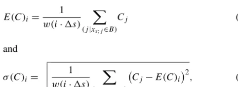
To characterize a property Cin the distance classi, we can calculate the expected value E(C) and standard deviation σ (C), taking only those values ofC into account that are situated in the boundaries of the distance classes:

E(C)i =

1 w(i·1s)

X

(j|xs;j∈B)

Cj (2)

and

σ (C)i=

v u u t

1 w(i·1s)

X

(j|xs;j∈B)

Cj−E(C)i

2

, (3)

where w(i·1s) represents the number of values (or grid cells) within the class. Please note that w(x) is the non-normalized value of the area function (Snell and Sivapalan, 1994). To visualize the proposed function, a simple synthetic basin with its stream network, distance classes, and an arbi-trary characteristic are shown in Fig. 3. To keep things simple Fig. 3c shows the unified flow length (comprisingxSandxH) derived from the flow direction data in Fig. 3b. As can be seen in Fig. 3c the basin has been split into five distance classes. Applying Eqs. (1) and (2) to the data (Fig. 3a) produces the average and standard deviation within these five distance classes. The obtained distance-factor function is shown in Fig. 4.

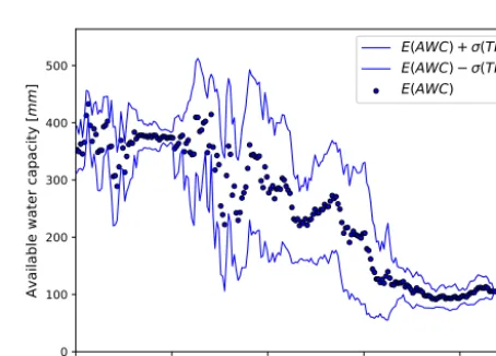
Figure 5 shows the application to real data in a meso-scale catchment, namely for AWC in the Mulde catchment. Expected values and a 1-σ range were plotted against the streamflow distance to the outlet. Distance classes with lower and higher variance are clearly visible in this figure as well as the succession of lower values to higher expected AWC values with increasing streamflow lengths.

Taking this approach we will be able to assess the arrange-ment of catcharrange-ment properties with the flow path which will, in the case of a non-random arrangement, be referred to as the spatial organization of the basin. Please note that we will always co-notate which type of distance-factor function (ex-pected value or standard deviation) has been applied. 3.2 Tools for automated sub-basin ascertainment The example of a distance-factor function in Fig. 5 shows that in some distance classes the AWC values are at a similar level due to a low standard deviation. This could be caused by the small size of the distance class (which is the case close to

the outlet and in the furthest distance class), but also by the fact that the class is located in the same region (low lands, mountainous regions). The example also shows that distance classes between 50 and 170 km are more heterogeneous, rec-ognizing its higher standard deviations. In order to minimize heterogeneity in these regions, a further subdivision is re-quired in these parts of the catchment.

To ensure more homogeneous sub-basins, an algorithm was developed based on consisting of the following.

1. An objective function which identifies the needs and (if necessary) the region of further subdivisions.

2. A tool to specify the subdivision points in the selected region for subdivision of the catchment.

3. An evaluation strategy to assess performed subdivi-sions.

The following subsections give a brief introduction to these three functionalities, before the sequence of the algo-rithm is described. More details on the introduced tools have been listed in Appendix A.

3.2.1 Objective function

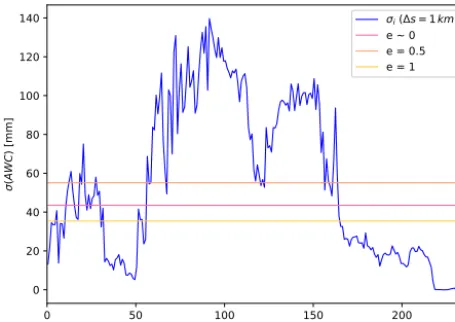
As outlined before, the standard deviationσ (C)can be used as an indicator of the heterogeneity of the sub-areas. Look-ing at the results of the distance-factor function forσ(AWC) of the Mulde (Fig. 6), the 1·σ (C) range clearly indicates regions with higher heterogeneity. These regions should be considered for subdivision. In order to build this into the GIS-based algorithm, a threshold value  was introduced that states whether a distance class is to categorize by (rel-atively) “low” or “high” standard deviations. The threshold is derived from the data by

=

NS

P

i=1

ωe_i·σ (C)i NS

P

i=1 ωe_i

, (4)

whereNSis the number of distance classes in the basin, the

exponenteis the parameter of a (non-)linearity factor, andω is a weighting factor defined as

ωi =

σ (C)i−1≤maxj≤NS σ (C)j

min

1≤j≤NS σ (C)j

₋ max

1≤j≤NS σ (C)j

. (5)

The actual objective function Z is the number of distance classes that display a standard deviation higher than the threshold. It is defined as the cardinality of the set of dis-tance classes fulfilling this condition:

Z= |[i|0≤i≤NS;σ (C)i> ]| →min. (6)

(c) Distance classes (b) Base data of synthetic catchment

(a) Input data

Figure 3.Exemplary input data(a), flow direction and Strahler order(b), and distance data and – classes(c).

Figure 4. Distance-factor function of sample data in a synthetic catchment.

requiring a further spatial subdivision. If the standard devi-ation in coherent distance classes stays below the threshold, these regions will be marked as low-variance regions.

As the index NS in Eq. (3) indicates, the thresholdis

calculated for the entire catchment and does not necessar-ily represent the true value of σ (C)for homogeneous sub-basins. It just helps to distinguish regions of high and low variances. Therefore it is recommended to vary the value of the non-linearity factorein a range of [0;∞], though values between 0 and 1 were found to be most applicable in our case studies. Ifeis set to 0,is equal to the average ofσ (C)in

f

Figure 5.Distance-factor function of AWC in the Mulde catchment.

Figure 6.Distance-factor function ofσ(AWC) and threshold values for different values ofe, in the Mulde catchment.

3.2.2 Subdivision tools

The functionality of the proposed tools will be shown for the synthetic catchment (Fig. 3) introduced in the previous sections (more details in Appendix A). The application of the objective function was expected to result in one of the listed three potential outcomes:

1. the standard deviations in all distance classes stay below threshold;

2. only parts of the classes have values ofσ (C) smaller than; and

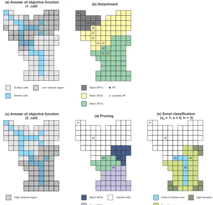
3. standard deviations of all classes are larger than. The first listed outcome would indicate that no further sub-division is required. The second would indicate that parts of the flow path display nearly homogeneous characteristics. This case is shown in Fig. 7a. Hatched cells indicate the low-variance region. Since this region is homogeneous it will not require any further handling and can be separated from the residual, more heterogeneous parts of the basin.

To do so, a tool called Detachmenthas been developed. The tool will determine the ideal drainage points ensuring their watershed covers the maximum range of low-variance regions. The identification of these separation points is done iteratively close to the transition from low-variance to high-variance regions. In Fig. 7b the result of Detachment is shown for the introduced synthetic catchment. Black dots in-dicate the identified drainage points; hollow points inin-dicate potential separation points which were rejected in the course of iterations. After applying theDetachmenttool, three sub-basins are defined, one containing the low-variance regions not requiring any further treatment and two sub-basins con-taining the remaining parts of the catchment.

Both remaining heterogeneous sub-basins, in this exam-ple, consist of distance classes with standard deviations

above the threshold. This could be caused by different spatial patterns in the sub-areas. On the one hand, parallel streams, or more specific neighbouring valleys with different vegeta-tion, slopes, etc., could cause higher variance. On the other hand, a zoning of hillslopes and higher elevated parts of the basin framing the drainage network (e.g. gley horizons close to streams) could result in higher values of the standard devi-ations. Such patterns are a result of the co-evolutional forma-tion of catchments (Blöschl et al., 2013; Sivapalan, 2005).

Further tools were developed specifically for these two dif-ferent potential root causes of heterogeneity. The first tool will provide a subdivision at stream branches (because our perspective of analysis is directed upstream; downstream would mean confluences) which will define new sub-basins at branching points of higher-order streams. Thepruningtool identifies branches by distance-factor functions of flow accu-mulation (see Appendix A).

The second tool is azonal classificationscheme, designed to account for heterogeneity within a distance class that is not caused by neighbouring valleys. We classified three zone types with an individual extent determined iteratively subject to three variables, i.e. Strahler order, distance to stream (com-parexH, Sect. 3.1), and heights. The first zone type, “close to

stream”, will be determined by the Strahler order and is in-tended to cover the stream network. Individual streams (be-ginning at the highest Strahler order and adding lower orders successively) and its extent (distance to the stream, begin-ning with 1·1o) close to stream zones are determined itera-tively, as already mentioned. The second zone type, referred to as “transition” zones, is first defined as all cells of the sub-basins not “close to streams”. Subsequently, these cells are reassigned by their height value either into “high-elevation” (heights above the iterated threshold) or “transition” (heights below threshold) zones. The height threshold mentioned be-fore is iteratively determined as the quantile of the histogram of height of all non-“close to stream” zones.

In Fig. 7d and e the results of an application of both tools for the exemplary synthetic catchment are shown. Hatched cells in the lower left area indicate high-variance regions that require partition. Thepruningresulted in two additional drainage points and split this region into three sub-basins. The zonal classification provided no new drainage points but specified three zones for the previously defined drainage points. Note that the algorithm has the potential to reject a zonal classification if the resulting variance is equal to or higher than that of the un-classed sub-basin. In this case all cells will be marked as “None” zones.

The introduced tool names will be used in Sect. 3.3 (and Fig. 8) where a detailed description and explanation of the algorithms’ sequence will be provided.

3.2.3 Evaluation scheme

Figure 7. (a, c)Answers of the objective function; result of(b)detachment,(d)pruning, and(e)zonal classification in the synthetic catch-ment.

i.e. minimizing heterogeneity through the introduction of sub-basins and zones. Since our assessment of heterogene-ity was based on the evaluation of distance classes, we could also define our objective as the minimization of the standard deviation within each distance class. No matter which tool has been applied, in some or all distance classes of the orig-inal sub-basinU multiple sub-basin/zones are present after-wards. Since the standard deviation was calculated for each partition unit (sub-basin or zone) individually, we were able to calculate the average standard deviation of neighbouring units within a distance class. This evaluation technique can be described as follows.

– Bspecifies the number of sub-basins defined within the original catchmentU.

– As a first step we estimated the standard deviationσ (C) (Eq. 2) within each sub-basin within distance classes based on flow length to the outlet of this sub-basin. As a second step the calculatedσ (C)values were transferred to the flow-length axis of the original watershedU. – This was done for all sub-basins by adding the

stream-flow length between their points of confluence and the outlet of the basin.

Figure 8.Sequence of the ACS algorithm.

σS(C)i=

1

Pi

P

p=1

w(i·1s)p

·

Pi

X

p=1

σ (C)i;p·w(i·1s)p, (7)

withPi being the number of parallel basins or zones,

w(i·1s)pthe number of cells within the distance class

i of the considered parallel basin/zoneb, andσ (C)i;p

the neighbouring standard deviations.

The success of the partition can be measured by compar-ison with the standard deviation of the unseparated basin σU(C), e.g. as the quotient of these values. With the new

valueσS(C)the effect of each subdivision can be measured independently of the objective function (and its threshold). 3.3 Sequence of the algorithm

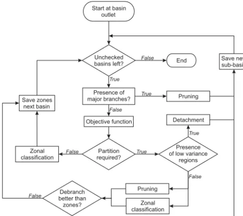
The tools presented above are at this point incoherent. Their sequential application in the ACS (Ascertainment by Catch-ment Structure) algorithm will be explained step-by-step fol-lowing the sequence shown in the flowchart in Fig. 8. Our considerations leading to the presented sequence can be sum-marized as follows.

1. Homogeneous regions should be separated from the re-maining basin by the algorithm.

2. Preferably a basin should be subdivided into sub-basins at major branches/confluences of the river network. 3. For high-variance regions the two optionspruningand

zonal classification should be carried out simultane-ously, since the origin of the high variance is unknown.

4. The results of both techniques (pruningor zonal clas-sification) should subsequently be compared with the subdivision yielding a lowerσS(C) to be saved (other results to be discarded).

5. Zonal classificationto be additionally applied in cases where only low-variance regions are present. Indepen-dent of the target to reduce σ (C), this way all ascer-tained sub-basins would obtain a zonal classification. At the very beginning of the sequence, on initialization of the algorithm, we would consider just one drainage point, i.e. at the outlet of the basin. After calculation of its watershed and the determination of the width function of accumulated partial areas, we would evaluate whether we also needed to consider major branches (see the Appendix for a detailed description of this procedure). Major branches would ac-count for larger, main rivers within a catchment. Since large rivers consist of a large number of cells draining into them, branches/confluences of rivers can be easily differentiated by size. If the test for major branches turns out to be true, the

pruning tool is called to specify two new drainage points (sub-basin outlets). These would be saved and put on the schedule of the algorithm for later examination.

Should a subdivision occur, the algorithm would start again at the previously used point, this time only looking at the watershed between the previous and newly defined drainage points. If no further major branch is present, the algorithm calculates the standard deviations of the charac-teristic of interest and the objective function to estimate the number of distance classes above the threshold.

There are three potential outcomes (see Sect. 3.2.2), i.e. standard deviation in none, some, or all classes above a threshold. For each outcome the algorithm had an option.

– If no standard deviation of a class is above, no fur-ther partition would be required so that the analysis of this part of the basin was complete and subsequently thezonal classificationwould be started and its results saved. The algorithm would then proceed and examine the next drainage point on its schedule.

– If only some classes are above , a partition would be required, but not in all areas. These areas would be clipped by thedetachmenttool. One or more new drainage points would be defined and added to the schedule. The algorithm would then start again at its last active point.

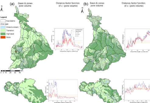
Figure 9.Results of ACS application for catchments of the Mulde and Regen, sub-basins based on pore volume(a)and slope(b). Comparison ofσU(C)andσS(C)for each application (red and blue lines).

This process would be repeated until all drainage points have been examined by the algorithm. The fact that each basin, or sub-basin, is analysed again after each subdivision provides the opportunity to apply a pre-partition. This could be useful if an existing structure (like a gauging network) is analysed for further improvements or just for zonal classifi-cation.

4 Method analysis

In this section we will analyse the outcome of applying the proposed algorithm for our case study catchments. First, we will take a qualitative look at the ascertained sub-basins and zones to assess similarities between catchments and charac-teristics. Subsequently we will take a quantitative look at the performance of the algorithm relative to its intended func-tion.

The ACS algorithm has been applied to all four catchments for pore volume and surface slope. Ascertained sub-basins and zones are shown in Figs. 9a–d (Mulde and Regen) and Fig. 10a–d (Main and Salzach). Additionally, the

distance-factor functions for standard deviationσ (C)for the respec-tive characteristicC, prior to and after partition of the catch-ment, are shown.

4.1 Qualitative evaluation

Looking at the results it can be noted that the proposed zonal classification was applicable to almost all catchments. Just one sub-basin in the Mulde catchment rejected a zonal classification (Fig. 9a, red sub-basin). Additionally, the de-fined sub-basins for both characteristics (same catchment) are comparable and often identical. This is mostly caused by the subdivision at a major branch. Nevertheless, differences in the number and extent of defined sub-basins are visible. More important though are the similarities and dissimilari-ties of the defined zones.

CTS zones for pore volume and comparing them to the maps of pore volume (Fig. 2), we can see a pattern across all catch-ments. Especially in the Mulde and Salzach catchments very narrow CTS zones have been defined for most parts of the basin. The occurrence of these narrow zones coincides with the presence of belts of different pore volumes around major streams (best visible in the Mulde catchment, Fig. 2, middle region). The soil patterns are not visible in the Regen and play a minor role in the Main catchment; hence, the distribu-tion of CTS zones is more likely to be extensive.

The same analysis for surface slope zones shows that these zones are in most cases more extensive than the pore-volume zones and follow the valley structure of the DEM (Fig. 1). CTS zones cover the streams and floodplains at the bot-tom the valleys, “transition” zones cover the hillslopes, and “high-elevation” zones cover higher located plains.

The interaction of zonal extent is best visible in the Salzach catchment, which is the most diverse in all of its characteristics (very high mountains with high slopes, soils with high and nearly no storage capacity). A comparison of the outcome for pore volume and slope (Fig. 9c, d) with the respective maps (Figs. 1 and 2) shows that the “ high-elevation” zones for pore volume cover the bare soil and rock formations with nearly no pore volume, and in the case of slope application the higher elevated parts of the mountains with only little slope. “Transition” zones cover in this case the steep hillslopes between the (comparably) flat valley bot-toms and high plateaus. In the case of pore volume they cap-ture the mid-range soils between the mountain top and the floodplains which are in both applications encompassed by CTS zones.

From this analysis of spatial natural patterns and patterns in the ascertained sub-basins and zones, we can draw the con-clusion that the outcome of the ACS algorithm is linked to the spatial organization of the considered catchment.

4.2 Quantitative evaluation

Having confirmed that the proposed algorithm can actually mirror the spatial organization of the catchment, we will now evaluate whether the heterogeneity of the specific character-istic has been decreased. As stated in Sect. 2.4 the intended function of the algorithm was the reduction of the number of distance classes comprising a standard deviationσ (C)above the threshold(of the characteristicC). To evaluate the per-formance towards this target we will look at the reduction of σ (C), defined as the normalized sum of allNSdifferences of

the standard deviation of the unseparated catchment σU(C)

and the separated basinσS(C):

α1=

NS

P

i=0

σU;i(C)−σS;i(C) NS

P

i=0 σU;i(C)

. (8)

The standard deviation of the separated catchmentσS(C)is calculated according to Eq. (6). In addition to this we applied a second performance metric to evaluate to what extent our target has been met. The metricα2highlights cases where the total heterogeneity was decreased significantly but was still above the objective as defined by threshold. The metricα2 was calculated as the delta between thresholdand the stan-dard deviation in the separated catchmentσS(C), normalized by the delta betweenand the standard deviation in the un-separated catchmentσU(C):

α2=

P

i∈M(S)

−σS;i(C)

P

j∈M(U )

−σU;j(C)

. (9)

In Eq. (8)Mis the set of distance classes comprising a higher standard deviation than the threshold:

M= [i|0≤i≤NS;σi≥]. (10)

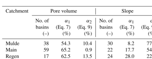
Performance data for all applications were listed in Table 1, including the number of ascertained sub-basins (demonstrat-ing modell(demonstrat-ing/calibration efforts).

As already indicated in the distance-factor functions of σ (C)(Fig. 9 and 10), the performance of pore volume ap-plications in all cases (and both evaluation subjects) was superior to slope applications, leading to a 2 to 6 times higher level of reduction (between 46 and 65 % total reduc-tion of variance). The remaining variance above the threshold ranged between 0.9 and 25 % for pore volume applications. Compared to slope applications this was better between 8 ppt (Regen) and 67 ppt (Mulde). Although the reduction of vari-ance for slopes might be inferior, up to 25 % of the varivari-ance could be compensated for by the ACS partition of the basin.

Focusing on cases with insufficient variance reduction, we were able to identify some limitations of the algorithm. First we will look at the slope application. The achieved reduction was generally low and the remaining variance was still high, but especially the outcome of the Mulde basin is inferior to all other (slope) applications.

Figure 10.Results of ACS application for catchments of the Main and Salzach (from top to bottom), sub-basins based on pore volume(a)and slope(b). Comparison ofσU(C)andσS(C)for each application (red and blue lines).

Table 1.Results of applications of ACS. Number of ascertained sub-basins and normalized reduction of standard deviation.

Catchment Pore volume Slope

No. of α1 α2 No. of α1 α2

basins (Eq. 7) (Eq. 9) basins (Eq. 7) (Eq. 9)

(–) (%) (%) (–) (%) (%)

Mulde 38 54.3 10.4 30 8.2 77.9

Main 59 65.2 0.9 22 17.7 54.3

Regen 17 62.5 13.5 24 28.0 22.1

Salzach 24 48.5 25.6 38 15.1 56.0

Another inferior case is the pore volume application in the Salzach basin. The shape of the basin as well as the amount of variation (see Fig. 10) cannot be explained as previously. Figure 10 shows the map of the AWC in the Salzach basin on a lower scale and the distance-factor function for standard de-viation of AWC. On the map red boxes highlight spots within the basin displaying much higher AWC values than its sur-rounding areas. These spots are also visible in the distance-factor function. For the separated basin (red line) the peaks are still visible after the separation, although the basic height of the line has been lowered. This observation can only be in-terpreted such that the occurrences of such soil enclosures are

a limiting factor for the reduction of heterogeneity with the ACS algorithm. It does not restrict its applicability, though. 4.3 Dependence on basin structure

consid-0 510 20 30 40km

AWC (2 m) [mm]

Max.: 780 Min.: 0

1

2

3

1

2

₃

Figure 11.AWC of the Salzach catchment and the distance-factor function ofσU(C)andσS(C). Red marked and numbered areas

incorpo-rating high-value enclosures.

Mulde

Resampled AWC (2 m) [mm]

Max.: 780

Min.: 20

Salzach

Resampled AWC (2 m) [mm]

Max.: 471

Min.: 94

0 10 20 40 60 80km

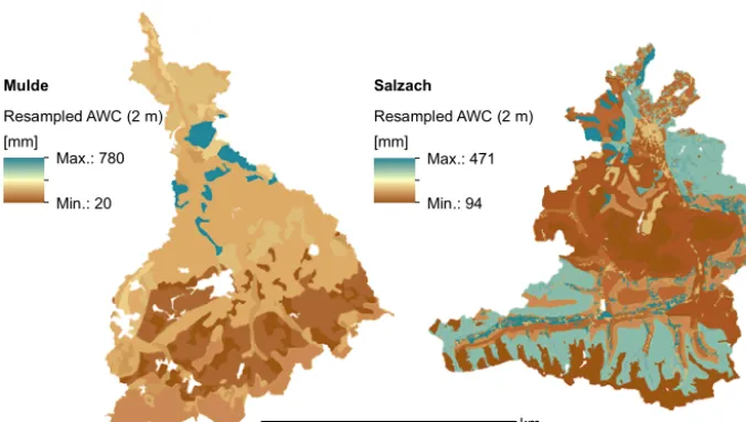
Figure 12.Resampled AWC values for the Mulde and Salzach catchments.

ered characteristics or the spatial arrangement/basin shape that caused the issue? In other words: if we could examine the same basin with another set of values, would the outcome, i.e. the number of sub-basins, zonal extent, and performance criteria change?

The problem is that no basin is like another, and even parts of the basin display different structures and shapes than the entire basin. Therefore, it is unlikely that there is only a sin-gle causal factor for the noticed performance decrease.

To overcome this issue we performed what we called a “resampling experiment”. The intention was to examine the same basin shape and spatial arrangement with a different set of values (just like a time series analysis). Therefore a quantile exchange of values has been performed.

Due to their similar sizes, the basins of the Mulde and Salzach have been chosen for resampling. First we took the maps for AWC of both basins (Salzach Fig. 1, Mulde not shown but the spatial organization is analogous to TPV, range of values from 51 to 471 mm) and calculated an empirical distribution function for each basin. Subsequently, the AWC values were replaced with their respective empirical quan-tile level. Finally, the distribution functions were exchanged (Mulde to Salzach, and vice versa) and the quantile levels were replaced with the exchanged distribution function quan-tiles. Results are shown in Fig. 12. We repeated this proce-dure with the DEMs as the source data for surface slopes.

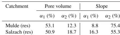
Table 2.Normalized reduction of standard deviation for resampled basins.

Catchment Pore volume Slope

α1(%) α2(%) α1(%) α2(%)

Mulde (res) 53.1 12.3 8.8 75.4

Salzach (res) 50.9 18.7 16.3 55.3

equipped with mid-range mountainous heights and more ho-mogeneous soil. That way we were able to assess the same basin shape and spatial arrangement with different (natural reasonable) ranges of parameter values.

The ACS algorithm has been applied to the resampled values of pore volume and surface slope. Ascertained sub-basins, zones, and distance-factor functions of the respective standard deviation are shown in Fig. 13; performance values are tabulated in Table 2. In the case of the Mulde basin the outcome did not change significantly. Ascertained sub-basins (number and shape) as well as zonal extent were very similar to the original results; performance values were stable. It can be noted that the distance-factor function forσ(AWC) had a very different shape than in the original basin (Fig. 6).

Application to AWC in the Salzach basin showed a sig-nificant change in performance. While the total reduction decreased, the remaining variance above the threshold was 20 ppt lower than in the original basin. This is also visi-ble in the distance-factor function of σ(AWC). Compared to Fig. 11 it can also be noted that previous peaks close to the outlet and in the more distant parts of the basin disap-peared. This result could be explained by the missing en-closures which have been transmitted as high values to the Mulde basin. Here, the allocation of the highest values is not organized in enclosures but in the upper–middle area of the catchment (see Fig. 12) following a stream-orientated pattern. The peak of the standard deviation is clearly visi-ble in the distance-factor function of the unseparated resam-pled basin in Fig. 13, but the techniques of the ACS algo-rithm are able to encompass this structure. Hence, the reduc-tion of variance remained on the same level. We also experi-enced a change in performance for the slope. The exchange of height values led to a lower range of slope values and a lower amount of heterogeneity. These patterns resulted in all other applications in inferior α2 performances. Still, the geomorphologic structure of the basin remained unchanged and heterogeneity could be assessed by the algorithm (visible through unchanged total reduction).

In conclusion we can state that the actual spatial arrange-ment, or more specifically its spatial organization, defines the outcome of the algorithm. Since this was our initial in-tention, this can be noted as a positive study outcome. On the downside we had to recognize that patterns (in this case soil patterns) that do not follow the co-evolutional structure of a basin (between soil and streams) (Blöschl et al., 2013)

cannot be captured satisfactorily by the proposed algorithm. Furthermore, a spatially homogeneous variation structure of catchment characteristics, independent of its actual amount of variation, is also complicated to assess with the ACS algo-rithm. However, we were able to demonstrate that the pro-posed algorithm works well for catchment characteristics that offer wide range patterns (like soil properties). (In the Supplement to this article we substantiate this statement by applying the algorithm to hydraulic conductivity data; results are in accordance with results of pore volume.)

5 Method application

In the previous sections we have shown how the algorithm works, what results it produces, and what information about the basins we gained from its application. But we have not yet assessed how useful it is and what benefits it could pro-vide. We will address this topic in the following two sub-sections. In comparison to a common subdivision, we will first evaluate its reduction of variance and second show its benefits for designing a hydrological rainfall–runoff model. 5.1 Comparison to gauging networks

The most common subdivision scheme is based on the avail-able gauging network. On the one hand this is due to calibra-tion requirements and on the other hand it is the only source for a reasonable partition of the catchment. Obviously, exist-ing gaugexist-ing networks are a result of multiple considerations and requirements, e.g. of water management issues. In some parts of the basin it tends to be denser than required to catch the natural heterogeneity within a river basin, but other hy-drological aspects (e.g. scale problems) might not be consid-ered sufficiently in the network design.

Comparing sub-basins defined by hydrological networks by looking at the results of the ACS algorithm might show differences in the number of separation points. Such a com-parison might help to provide advice to decision makers on where to locate new gauges for reducing variances. It could also provide information about the usefulness of the ACS al-gorithm. (Please keep in mind that for the decision maker the usefulness of the algorithm might be limited by the informa-tional value of the specific catchment characteristic for runoff generation processes.)

Two benchmark subdivisions were established.

1. A subdivision based on the gauging network to be com-pared to the obtained ACS basins (without zones). 2. A subdivision based on the gauging network with an

Basin & zones pore volume

Basin & zones slope

Distance-factor function of (slope) Distance-factor function

of (pore volume)

Legend Sub-basins Zone type

Close to stream Transition High level None

0 510 20 30 40

km

(a)

(b)

Figure 13. Results of ACS application for resampled catchments of the Mulde and Salzach (from top to bottom) sub-basins based on resampled pore volume(a)and slope(b). Comparison ofσU(C)andσS(C)for each application (red and blue lines).

Gauging networks and defined land cover zones are shown on the left of Fig. 14. The distance-factor function of stan-dard deviations for pore volume (centre of Fig. 14) and slope (right) are displayed in addition to the results of ACS subdi-visions. Performance data were summarized in Table 3.

Looking at the distance-factor function for pore volume, it can be recognized that the red line, representing ACS results, is below the blue (representing gauges) and green (repre-senting gauges and land cover) lines for nearly all distances, demonstrating the advantage of ACS. The ACS advantage is also confirmed by the performance measures in Table 3. The total reductionα1(Eq. 8) exceeds the achieved values for gauges and land cover (bench-2) by a factor of between 1.3 and 1.8. Furthermore, the remaining variance above the threshold α2 (Eq. 9) is lower by between 16 and 45 ppt. Please note that this advantage was accomplished with a significantly smaller number of subdivisions. This makes us conclude that the proposed algorithm is a more effective tool to reduce the heterogeneity of pore volume data or any

catch-ment characteristic that has a similar spatial organization (see the Supplement).

Similarly to Sect. 4, results for slopes provided a differ-ent impression and quality. In the distance-factor functions (Fig. 14) we can see that all lines are on an equal level and show no clear advantage for any of the partition strategies. Looking at the performance results in Table 3, we can see that without zonal classification the gauging network has an advantage for ACS results. Especially the sub-divisions in the Mulde basin are ineffective. However, with the introduc-tion of zonal classificaintroduc-tion, the performance values are at a more comparable level, withα1 results ranging between 8 and 17 % (with the exception of the Regen catchment). Results for remaining variance, however, are more different (22–77 % ACS and 30–54 % bench-2), which points out that the benchmark partition captures the heterogeneity of slopes at least at some points of the basin better than the ACS.

Figure 14.Subdivisions based on gauging network and zonal classification and distance-factor functions ofσ (pore volume) andσ (slope) (left to right) for catchments of the Mulde, Main, Regen, and Salzach (top to bottom).

catchments in isolation will not capture the heterogeneity of surface slopes, and their performance is subject to a zonal classification that can be described as small-scale distributed and fragmented.

5.2 Modelling application

Our model of choice is the HBV96model (Lindström et al., 1997), due to the fact that we already used its recommended catchment zonal classification scheme, its obvious ability to incorporate zones, and, after all, due to its common usage.

Table 3.Normalized reduction of standard deviation for sub-basins based on gauging network, ACS basins, and gauges and land cover.

Catchment Pore volume Slope No. of gauges

α1(%) α2(%) α1(%) α2(%) Gauging network

Mulde 24.2 53.4 9.4 69.9 40

Main 41.9 26.2 14.0 44.0 46

Regen 21.1 74.6 10.1 57.9 20

Salzach 30.3 48.8 9.6 68.5 33

ACS basins only

Mulde 32.8 45.3 0.0 100.0 38/30 Main 50.7 8.5 9.2 72.9 59/22 Regen 40.9 35.9 14.1 52.8 17/24 Salzach 40.6 24.6 9.3 73.6 24/38 Gauging network and land cover Occurring zones

Mulde 35.3 35.0 14.5 54.8 2

Main 48.9 17.7 19.8 26.2 2

Regen 33.2 59.4 19.1 27.4 2

Salzach 38.4 50.1 21.6 30.8 3

lower groundwater storage. Since the modelling application is meant to be short, please see Lindström et al. (1997) for further information about the model.

Our application case was the Mulde catchment due to good data availability. Daily mean discharge, precipitation sums, temperature means, and sums of potential evapotranspiration time series from 1951 to 2011 are available for 39 gauged sub-basins (discharge data available for 20–39 gauges, de-pendent on the time window).

Two spatial model set-ups were employed for application; both are shown in Fig. 15. The left part of Fig. 15 shows the bench-2 partition we already used in the previous section, based on gauging network, heights, and land cover. In the right part of Fig. 15 our proposed subdivision of the catch-ment, based on gauging network and pore volume, is shown. The gauging network has been used as a pre-partition of the basin and the ACS refined the sub-basin density and defined zones for all sub-basins. We chose pore volume as the catch-ment characteristic. Its spatial organization has been incorpo-rated into the spatial set-up of the model. Our decision was based on the fact that ACS worked better for pore volume than for slope and that information about storage capacities seemed to be more valuable for a conceptual (storage-based) model.

Besides the incorporation into the model structure, we were able to use information about the catchment character-istics in the calibration process. Each (ACS) sub-basin fea-tured three zones, each having an individual average value for pore volume. Since we minimized the heterogeneity of the respective characteristic we were able to assume a uni-form distribution of this value for the entire zone. Now, an automated calibration routine benefitted from this

informa-tion and we were able to reasonably couple parameters of the zones by their respective average of the characteristic.

Say each zone included a parameter calledX. An algo-rithm, like the BOBYQA algorithm employed in this study (Powell, 2009), offers in each iteration step a guess for this parameterx˙. The parameter guess is then transformed to the zonal parameter by the zone characteristicEZone(C) normal-ized by the average value of the entire basinE(C)and a lin-ear coupling parameterkX:

XZone=

EZone(C)

E(C) ·kX· ˙x. (11)

Please note that the coupling parameter is subject to the cal-ibration process itself and is linked to a single parameter. In this study we coupled six zonal parameters that are related to soil properties. This coupling scheme (comparable to studies by Gharari et al., 2014) has additionally been applied to the benchmark. Here,E(C)in Eq. (10) is omitted and applied only to field zones, while forest zones use an unchangedx.˙ Since the coupling of the benchmark subdivision is not based on any process assumptions, we additionally applied a free parameterization where all parameters within each sub-basin and zone can be used for model fitting.

Figure 15.Spatial structures for the HBV96model:(a)ACS basins and zones;(b)gauging network, land use, and heights.

Table 4.Parameter quantities.

Benchmark Benchmark Benchmark ACS ACS

Free Six-coupled All coupled Six-coupled All coupled

Sub-basins 38 38 38 44 44

Zones per sub. ∼30 ∼30 ∼30 3 3

Parameter (total) 19562 12198 1710 2244 1980

Parameter (per sub.) ∼495 ∼321 45 51 45

Figure 16.Nash–Sutcliffe efficiency of the ACS-based model and benchmark model; six coupled parameters.

Besides this “lumped” evaluation, we compared the per-formance of the models at each gauge in each period. A comparison of NSE for a six-parameter-coupled model is shown in Fig. 16, and for ACS and a free-benchmark model in Fig. 17. Comparison for the all-coupled parameterization is shown in Fig. 18. We can see that the individual mances led to the same conclusion as the lumped

perfor-mance, though some results are better for benchmark mod-els (both parameterizations). To be more precise, in the case of the six-parameter-coupled model, 20 points (representing a single gauge in one of the time periods) are below equiv-alency (representing a better performance of the benchmark model), in the case of the free-benchmark model, 12, and for the all-coupled benchmark, 23 points, representing 15, 9, and 20 % of the evaluated cases.

In conclusion we had to ask ourselves: what is the result of this modelling study? Obviously, we could improve the modelling performance. In accordance with findings in the literature we could prove that additional information relevant to hydrological processes improves the model performance (Finger et al., 2015; Li et al., 2015) and, furthermore, we can confirm that the spatial organization of catchment character-istics (in this case pore volume) is relevant information. The latter conclusion is drawn from the fact that the ACS model offers a similar (or superior) model performance to the cou-pled model although it included fewer model parameters.

6 Conclusions

Table 5.Nash–Sutcliffe efficiencies of the benchmark and ACS model.

Simulation NSE_B;Free NSE_B;6 NSE_B;All NSE_ACS;6 NSE_ACS;All

(Start–end) (–) (–) (–) (–) (–)

1995–2006 (C) 0.678 0.659 0.682 0.792 0.791

2007–2011 (V) 0.524 0.570 0.578 0.622 0.647

1984–1995 (V) 0.496 0.516 0.525 0.607 0.546

1951–1961 (V) 0.433 0.568 0.458 0.660 0.572

Figure 17.Nash–Sutcliffe efficiency of the ACS-based model and benchmark model; free parameterization.

conceptual, semi-distributed hydrological models. First, we proposed the distance-factor function to assess the interac-tion of an arbitrary catchment characteristic with the flow path. Graphical representations of this function are capable of visualizing the heterogeneity of the considered character-istic. We further build an algorithm on this proposed func-tion, mainly focusing on factor functions of standard devia-tions, with the objective of reducing the heterogeneity of the respective catchment characteristic. The proposed ACS algo-rithm utilizes three different techniques to reduce the hetero-geneity that were developed by looking at the main sources of heterogeneity visible in natural catchments. The outcome of the algorithm offers a spatial subdivision of the catchment, at a minimum of standard deviation of the respective charac-teristic.

After the introduction of these methods we performed an extensive test of the ACS algorithm. First, we tested model functionality and its limits of application to four different basins. We evaluated the spatial patterns we obtained rela-tive to visible spatial patterns in the basins. Furthermore we compared the reduction of variance for different characteris-tics and basins. Next, we evaluated the usefulness of the ob-tained results. On the one hand we compared the variance re-duction to a benchmark separation and on the other hand we merged our results to a semi-distributed hydrological model.

Figure 18.Nash–Sutcliffe efficiency of the ACS-based model and benchmark model; all zonal parameters coupled.

The modelling study demonstrated the benefits we can gen-erate from incorporating the spatial organization of the basin. We were able to confirm that the distance-factor func-tion is a useful tool for detecting non-random spatial pat-terns and the interaction of catchment characteristics with the flow path. Furthermore, we could confirm its ability to detect anomalies in the structure of the catchment, e.g. spots of different soil types that do not follow the co-evolutional structure of the basin.

Our future work will focus on two topics: on the one hand, we have to further improve the subdivision algorithm. At this point we are able to assess the structure of a single character-istic, while it is highly desirable to consider multiple charac-teristics. Additionally we will have to develop methods to en-compass soil enclosures and fragmented characteristics. The latter problem might lead to the well-known HRU concept. We have to study whether such development is desirable. On the other hand, we will address the value for catchment similarity studies. Following intentions by Mesa and Mifflin (1986), who suggested the width function as an indicator of catchment similarity, it might be worthwhile to investigate how results of the distance-factor function can be used to characterize similarity.

Appendix A

In this Appendix details of the proposed ACS tools are given for further understanding of the algorithm. Each tool will be addressed separately.

A1 Detachment tool for low-variance regions

Regions of small variance have no need for further subdivi-sions; hence, they are detached from the rest of the basin. Since the exact allocation of these regions is known, all cells within can be defined as target area T (hatched in Fig. 7a). The remaining cells are drawn together as non-target area NT. If one random point of the basin is selected as a possi-ble separation point (SP) and its watershed is calculated, the set of points belonging to the watershed, or sub-basin, of SP, BSP, is obtained. The calculated watershed BSP covers parts of T and NT and hence a coverage rate can be calculated as the proportion of the cardinalities of the intersections and their respective superset:

OSP=

|BSP∩T| |T| −

|BSP∩NT|

|NT| , (A1)

which shall be maximized.

The objective of a detachment O is to find a separation point (SP) whose basin BSP covers a maximum of T and a minimum of NT. Please note that for regions located at the outlet of the basin or at its upstream boundary, only one SP will be defined. Possible SPs are assumed to be allocated at the transit of the main stream from T to NT, or vice versa. An iterative search returns the coverage values O and the highest value is selected as SP, defining a new sub-basin. In the upper part of Fig. 7a the obtained separation as well as the rejected SPs of the iteration (hollow points) are shown.

A2 Pruning at confluences/branches

To identify branches, the distance-factor function of flow ac-cumulation (i.e. the cumulative number of cells draining into a cell) (FAcc) is examined. FAcc indicates the contributing drainage area to each stream cell. Hence, discontinuities in the distance-factor function indicate confluences of streams (see Fig. A2 for an example of the distance-factor function). Beginning at the outlet (0 on thex-axis), two features are visible: a slowly decreasing line of high FAcc values, repre-senting the main stream at the outlet, and a noise-like smaller range of FAcc values close to the abscise, caused by the smaller tributary streams and contributing areas. To identify major tributaries, this noise has to be removed. We assume that in the first distance class the disparity between main rivers and contributing hillslopes is most distinct. Within the first class a k-means cluster analysis is carried out to divide high and low FAcc values. The threshold value τS is

deter-mined as

τS=min_c maxc1[FAcc];maxc2[FAcc]

·1− γ 10

, (A2)

Figure A2.Distance-factor function of flow accumulation in the catchment of the Mulde.

wherec1andc2indicate the clusters andγ is the reduction order and by default 0. The algorithm will start with the de-fault value forγ and searches for the first branch in the up-stream direction. If no branch is found, the order γ is in-creased by 1. The maximum order is set to 10. Please note that the higherγ is set, the lower the threshold gets, and the more FAcc values remain for analysis. The routine identifies the coordinates of the branch inducing the drop in FAcc val-ues (see Fig. A2, for example at distance≈80 km).

Drainage points of major streams or major stream branches are identified likewise. Before the objective func-tion is called, prevailing FAcc values in the basin are checked. If the FAcc value of the tributary stream is higher than the threshold valueτR, a subdivision is performed. This

parameter is calculated as a percentage of the maximum FAcc value in the entire watershed (e.g. 5 %) once at the ini-tialization of the algorithm.

A3 Zonal classification

The iterative search for the optimal zonal classification in-volves three parameters: reduction of Strahler ordersR, dis-tance from streamo, and height quantile h. The maximum Strahler order within the considered sub-basin mS is also in-volved, but it is a constant. Initial values aresR=0, o=0,

andh=0/hite (note that hite is a required user-defined rameter > 1). In each iteration step one of the three pa-rameters is increased to its maximum value (sR;Max=mS; oMax=5;hMax=hite), creating a different composition of the zonal extent.

sR controls which cells within the basin are potential

“close to stream” (CTS) zones. All stream cells of Strahler order greater than/equal to mS-sR and all non-stream cells

odefines the width of CTS zones. All potential CTS cells withxH≤o·1o(as defined in Sect. 3) are confirmed as CTS cells; all remaining cells of the sub-basin are “transition” (TS) cells.

h controls the threshold used to define “high-elevation” (HE) zones. An empirical distribution function of heights (taken from the input DEM) of all FFS cells is calculated. The height thresholdτHis then calculated as theh/hite·100 (%) quantile of the empirical distribution function. All cells with an assigned height >τH are defined as HE zones; all remaining cells are confirmed as TS cells.

The Supplement related to this article is available online at https://doi.org/10.5194/hess-21-4259-2017-supplement.

Competing interests. The authors declare that they have no conflict of interest.

Acknowledgements. The authors would like to thank the editor and all reviewers for their comments that helped to improve this article.

Edited by: Günter Blöschl

Reviewed by: three anonymous referees

References

Band, L. E.: Topographic Partition of Watersheds with Dig-ital Elevation Models, Water Resour. Res., 22, 15–24, https://doi.org/10.1029/WR022i001p00015, 1986.

Beven, K. J. and Kirkby, M. J.: A physically based, vari-able contributing area model of basin hydrology/Un mod-èle à base physique de zone d’appel variable de l’hydrologie du bassin versant, Hydrological Sciences Bulletin, 24, 43–69, https://doi.org/10.1080/02626667909491834, 1979.

Beven, K. J., Kirkby, M. J., Schofield, N., and Tagg, A. F.: Testing a physically-based flood forecasting model (TOP-MODEL) for three U.K. catchments, J. Hydrol., 69, 119–143, https://doi.org/10.1016/0022-1694(84)90159-8, 1984.

Blöschl, G., Sivapalan, M., Wagener, T., Viglione, A., and Savenije, H.: Runoff Prediction in Ungauged Basins: Synthesis across Pro-cesses, Places and Scales, Cambridge University Press, Cam-bridge, 492 pp., 2013.

Bossard, M., Feranec, J., and Otahel, J.: CORINE land cover tech-nical guide: Addendum 2000, EEA, Copenhagen, 2000. Bremicker, M.: Das Wasserhaushaltsmodell LARSIM:

Modell-grundlagen und Anwendungsbeispiele, Hochwasserzentralen LUBW, BLfU, LfU RP, HLNUG, BAFU, 2016.

D’Odorico, P. and Rigon, R.: Hillslope and channel contribu-tions to the hydrologic response, Water Resour. Res., 39, 1113, https://doi.org/10.1029/2002WR001708, 2003.

Dunn, S. M. and Lilly, A.: Investigating the relationship between a soils classification and the spatial parameters of a conceptual catchment-scale hydrological model, J. Hydrol., 252, 157–173, https://doi.org/10.1016/S0022-1694(01)00462-0, 2001. Finger, D., Vis, M., Huss, M., and Seibert, J.: The value

of multiple data set calibration versus model complexity for improving the performance of hydrological models in mountain catchments, Water Resour. Res., 51, 1939–1958, https://doi.org/10.1002/2014WR015712, 2015.

Flügel, W. A.: Delineating hydrological response units by ge-ographical information system analyses for regional hydro-logical modelling using PRMS/MMS in the drainage basin of the River Bröl, Germany, Hydrol. Process., 9, 423–436, https://doi.org/10.1002/hyp.3360090313, 1995.

Gharari, S., Hrachowitz, M., Fenicia, F., and Savenije, H. H. G.: Hydrological landscape classification: investigating the

perfor-mance of HAND based landscape classifications in a central European meso-scale catchment, Hydrol. Earth Syst. Sci., 15, 3275–3291, https://doi.org/10.5194/hess-15-3275-2011, 2011. Gharari, S., Shafiei, M., Hrachowitz, M., Kumar, R., Fenicia,

F., Gupta, H. V., and Savenije, H. H. G.: A constraint-based search algorithm for parameter identification of envi-ronmental models, Hydrol. Earth Syst. Sci., 18, 4861–4870, https://doi.org/10.5194/hess-18-4861-2014, 2014.

Grayson, R. and Blöschl, G. (Eds.): Spatial patterns in catchment hydrology: Observations and modelling, Cambridge Univ. Press, Cambridge, 404 pp., 2001.

Gupta, V. K. and Mesa, O. J.: Runoff generation and hydro-logic response via channel network geomorphology — Re-cent progress and open problems, J. Hydrol., 102, 3–28, https://doi.org/10.1016/0022-1694(88)90089-3, 1988.

Gupta, V. K., Waymire, E., and Wang, C. T.: A repre-sentation of an instantaneous unit hydrograph from geomorphology, Water Resour. Res., 16, 855–862, https://doi.org/10.1029/WR016i005p00855, 1980.

Jenson, S. and Domingue, J.: Extracting topographic structure from digital elevation data for geographic information-system anal-ysis, Photometric Engineering and Remote Sensing, 54, 1593– 1600, 1988.

Kirkby, M. J.: Tests of the random network model, and its appli-cation to basin hydrology, Earth Surf. Processes, 1, 197–212, https://doi.org/10.1002/esp.3290010302, 1976.

Lai, Z., Li, S., Lv, G., Pan, Z., and Fei, G.: Watershed delineation using hydrographic features and a DEM in plain river network region, Hydrol. Process., 30, 276–288, https://doi.org/10.1002/hyp.10612, 2016.

Li, H., Xu, C.-Y., and Beldring, S.: How much can we gain with increasing model complexity with the same model concepts?, J. Hydrol., 527, 858–871, https://doi.org/10.1016/j.jhydrol.2015.05.044, 2015.

Lindström, G., Johansson, B., Persson, M., Gardelin, M., and Bergström, S.: Development and test of the distributed HBV-96 hydrological model, J. Hydrol., 201, 272–288, https://doi.org/10.1016/S0022-1694(97)00041-3, 1997. Mesa, O. J. and Mifflin, E. R.: On the relative role of Hillslope and

Network Geometry in Hydrologic Response, in: Scale Problems in hydrology: runoff generation and basin response, edited by: Gupta, V. K., Scale Problems in hydrology, 2, Reidel, Dordrecht, 1–19, 1986.

Moore, I. D. and Grayson, R. B.: Terrain-based catchment partition-ing and runoff prediction uspartition-ing vector elevation data, Water Re-sour. Res., 27, 1177–1191, https://doi.org/10.1029/91WR00090, 1991.

Müller, C., Hellebrand, H., Seeger, M., and Schobel, S.: Identifica-tion and regionalizaIdentifica-tion of dominant runoff processes – a GIS-based and a statistical approach, Hydrol. Earth Syst. Sci., 13, 779–792, https://doi.org/10.5194/hess-13-779-2009, 2009. Nash, J. E. and Sutcliffe, J. V.: River flow forecasting through

con-ceptual models part I – A discussion of principles, J. Hydrol., 10, 282–290, https://doi.org/10.1016/0022-1694(70)90255-6, 1970. Nobre, A., Cuartas, L., Hodnett, M., Rennó, C.,

Powell, M.: The BOBYQA algorithm for bound constrained opti-mization without derivates, Department of Applied Mathematics and Theoretical Physics, Cambridge, 2009.

Rigon, R., Bancheri, M., Formetta, G., and de Lavenne, A.: The geomorphological unit hydrograph from a historical-critical perspective, Earth Surf. Proc. Land., 41, 27–37, https://doi.org/10.1002/esp.3855, 2016.

Rinaldo, A., Marani, A., and Rigon, R.: Geomorpho-logical dispersion, Water Resour. Res., 27, 513–525, https://doi.org/10.1029/90WR02501, 1991.

Robinson, J. S., Sivapalan, M., and Snell, J. D.: On the rel-ative roles of hillslope processes, channel routing, and network geomorphology in the hydrologic response of natural catchments, Water Resour. Res., 31, 3089–3101, https://doi.org/10.1029/95WR01948, 1995.

Rodríguez-Iturbe, I., and Valdés, J. B.: The geomorphologic struc-ture of hydrologic response, Water Resour. Res., 15, 1409–1420, https://doi.org/10.1029/WR015i006p01409, 1979.

Schumann, A., Funke, R., and Schulz, G.: Application of a geographic information system for conceptual rainfall-runoff-modeling, J. Hydrol., 290, 45–61, 2000.

Sivapalan, M.: Pattern, Process and Function: Elements of a Uni-fied Theory of Hydrology at the Catchment Scale, in: Encyclope-dia of hydrological sciences, edited by: Anderson, M. G., Wiley, Chichester, 193–219, 2005.

Snell, J. D. and Sivapalan, M.: On geomorphological dis-persion in natural catchments and the geomorphologi-cal unit hydrograph, Water Resour. Res., 30, 2311–2323, https://doi.org/10.1029/94WR00537, 1994.

Soulsby, C., Tetzlaff, D., Rodgers, P., Dunn, S., and Wal-dron, S.: Runoff processes, stream water residence times and controlling landscape characteristics in a mesoscale catchment: An initial evaluation, J. Hydrol., 325, 197–221, https://doi.org/10.1016/j.jhydrol.2005.10.024, 2006.

Sponagel, H. (Ed.): Bodenkundliche Kartieranleitung: Mit 103 Tabellen und 31 Listen, 5., verb. und erw. Aufl, Schweizerbart, Stuttgart, 438 pp., 2005.

Verdin, K. and Verdin, J.: A topological system for delineation and codification of the Earth’s river basins, J. Hydrol., 218, 1–12, https://doi.org/10.1016/S0022-1694(99)00011-6, 1999. Vogt, J. V., Colombo, R., and Bertolo, F.: Deriving drainage