Analysis and modelling of a 9 3 kyr palaeoflood record: correlations, clustering, and cycles

https://doi.org/10.5194/hess-21-5547-2017 © Author(s) 2017. This work is distributed under the Creative Commons Attribution 3.0 License.

Analysis and modelling of a 9.3 kyr palaeoflood record:

correlations, clustering, and cycles

Annette Witt1, Bruce D. Malamud2, Clara Mangili3,a, and Achim Brauer3

1_{Max Planck Institute for Dynamics and Self-Organisation, Göttingen, Germany} 2_{Department of Geography, King’s College London, London, UK}

3_{GFZ German Research Centre for Geosciences, Potsdam, Germany}

a_{now at: Section of Earth and Environmental Sciences, University of Geneva, Geneva, Switzerland}

Correspondence to:Annette Witt ([email protected]) and Bruce D. Malamud ([email protected]) Received: 8 September 2016 – Discussion started: 21 October 2016

Revised: 2 July 2017 – Accepted: 17 July 2017 – Published: 14 November 2017

Abstract. In this paper, we present a unique 9.5 m palaeo-lacustrine record of 771 palaeofloods which occurred over a period of 9.3 kyr in the Piànico–Sèllere Basin (southern Alps) during an interglacial period in the Pleistocene (some-time from 780 to 393 ka) and analyse its correlation, clus-tering, and cyclicity properties. We first examine correla-tions, by applying power-spectral analysis and detrended fluctuation analysis (DFA) to a time series of the num-ber of floods per decade, and find weak long-range persis-tence: a power-spectral exponent βPS≈0.39 and an

equiv-alent power-spectral exponent from DFA, βDFA≈0.25. We

then examine clustering using the one-point probability dis-tribution of the inter-flood intervals and find that the palae-ofloods cluster in time as they are Weibull distributed with a shape parameterkW=0.78. We then examine cyclicity in

the time series of number of palaeofloods per year, and find a period of about 2030 years. Using these characterizations of the correlation, clustering, and cyclicity in the original palaeoflood time series, we create a model consisting of the superposition of a fractional Gaussian noise (FGN) with a 2030-year periodic component and then peaks over thresh-old (POT) applied. We use this POTFGN+Periodmodel to

cre-ate 2 600 000 synthetic realizations of the same length as our original palaeoflood time series, but with varying intensity of periodicity and persistence, and find optimized model pa-rameters that are congruent with our original palaeoflood se-ries. We create long realizations of our optimized palaeoflood model, and find a high temporal variability of the flood fre-quency, which can take values of between 0 and > 30 floods century−1. Finally, we show the practical utility of our

opti-mized model realizations to calculate the uncertainty of the forecasted number of floods per century with the number of floods in the preceding century. A key finding of our paper is that neither fractional noise behaviour nor cyclicity is suf-ficient to model frequency fluctuations of our large and con-tinuous palaeoflood record, but rather a model based on both fractional noise superimposed with a long-range periodicity is necessary.

1 Introduction

palaeo-lake Piànico–Sèllere (northern Italy), and construct a model to take into account the observed behaviour. In this introduc-tion, we present the idea of correlationsand clusteringin time series, and then summarize the overall organization of this paper.

We first consider correlationsin a time series. Consider an uncorrelated time series (e.g. a white noise), where val-ues are independent of one another, i.e. it is equally likely at each time step to have values above or below the median value. To illustrate correlations, take a flood intensity time series, with flood intensity the number of floods per year; a “flood” here might be defined in many different ways. If the flood intensity time series is uncorrelated, when there is a year with a large intensity (a large number of floods oc-curring, above the median number of floods), it is equally probable to have the next year a number of floods that is above or below the median, i.e. a flood intensity value that is “large” (more floods) or “small” (zero or few floods). In contrast, for a flood intensity time series that exhibits posi-tive correlations, adjacent values will have flood intensities that are on average closer to each other (in intensity) than for an uncorrelated time series; large values tend to follow large ones, and small follow small. Temporal correlations are also referred to as persistence or memory (see Witt and Malamud, 2013, and references therein). Two examples of positive cor-relations in time series are given in Fig. 1a and b, using a tree ring standardized growth index for Bristlecone pine, White Mountain, California, USA, for the years AD 0–1962 and cosmic ray neutron counts per hour, Beijing, China, 1 Jan-uary to 11 March 2008. In these two Fig. 1 panels, succes-sive values in both series are positively correlated with one another, and are examples of persistent time series.

Correlations can be both short-range (where only values in a time series close to each other are correlated) or long-range (where all values in the time series are correlated with one another). We will find that the unequally spaced palae-oflood time series used in this paper exhibit both long-range correlations and long period cyclical behaviour, and will fo-cus on long-range (vs. short-range) persistent models in this paper. Long-range correlations have been discussed and doc-umented for many processes in the environmental and Earth Sciences (see Box et al., 2013; Witt and Malamud, 2013, and references therein), with examples including river run-off and precipitation (Hurst, 1951; Mandelbrot and van Ness, 1968; Montanari et al., 1996; Koscielny–Bunde et al., 2006; Mudelsee, 2007; Khaliq et al., 2009; Ghil et al., 2011), at-mospheric variability (Govindan et al., 2004) and tempera-tures over short- to very-long timescales (Pelletier and Tur-cotte, 1997; Fraedrich and Blender, 2003). The idea of long-range correlations is commonly used to characterize obser-vational and experimental measurement data across many other scientific disciplines: For instance Peng et al. (1993b, 1994) found long-range persistence in the nucleotide organi-zation of DNA sequences, Kurths et al. (1995) detected long-range correlations in time series from radio astronomy, Peng

0 5000 10000 15000

D

aily

d

ischar

ge

(m

3s −1)

0 5000 10000 15000

1878 1888 1898 1908 1918 1928 1938 1948 1958 1968 1978 1988

D

aily

d

ischar

ge

(m

3s −1)

Year

1878 1888 1898 1908 1918 1928 1938 1948 1958 1968 1978 1988 Year

0 500 1000 1500 2000

0 500 1000 1500 2000

S

tandar

d

ized

tr

ee-gr

ow

th

Index (no

units)

520 530 540 550

01 Jan 08 15 Jan 08 29 Jan 08 12 Feb 08 26 Feb 08 11 Mar 08

Counts

per

hr

(thousands)

Calendar year

Date (a)

(b)

(c)

(d)

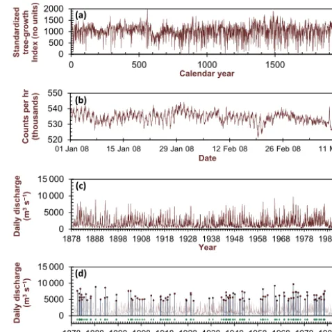
Figure 1.Example of correlations, clustering, and cyclicity (aand

bfollowing Witt et al., 2010). (a)Tree ring standardized growth

index for Bristlecone pine, White Mountain, California, USA, for

the years AD 0–1962 (Ferguson et al., 1994).(b)Cosmic ray

neu-tron counts per hour, Beijing, China, 1 January to 11 March 2008

(NGDC, 2008). In(a)and(b)successive values in each both

se-ries are positively correlated with one another, and are examples of

persistent time series.(c)Maximum daily discharge,Q, for station

05474500 on the Mississippi River at Keokuk, Iowa, for 116 water years, 1878–1993 with data from Slack and Landwehr (1992) and

USGS (2017) and described in Malamud et al. (1996).(d)

Partial-duration flood series, where floods are the largest 116 maximum

daily discharge from(c)over the 116-year period, with daily

dis-charges separated by at least 30 days to be considered a flood. In our partial duration series, 48 of the 116 years have 0 floods, 33 years have 1 flood, 26 years have 2 floods, and 6/2/1 years have 3/4/5 floods. The value of these maximum daily discharges for each flood event is projected to thex-axis (daily discharge=0 m3s−1). Below this is shown (green dots) all events along one line, an ex-ample of a data series that is strongly clustered in time. Clustering is due to (i) seasonal effects (cyclicity) and (ii) longer-term cycles.

et al. (1993a) and Penzel et al. (2003) analysed long-term recordings of heart rate variability.

or-Lake Iseo

(a)

0

2

4

6

8

Re

la

ti

ve

 a

ge

 [

ky

r]

(b)

(c)

65 yr 

gap

0 1 2 km

N

No. of detrital layers

per 100 varves

Figure 2.Site, sediment outcrop, and data.(a)Location of palaeolake Piànico–Sèllere, Italy. Underlying image © 2017 DigitalGlobe.(b)

Detail of the 9.5 m sediment outcrop containing a winter layer and parts of two summer layers with, shown here, a detrital layer that is

interpreted as a flood event.(c)Graphical representation of the sediment outcrop with the grey horizontal lines indicating detrital layers,

brown horizontal bars indicating the number of detrital layers per decade and the striped bar showing a 65-year gap (see Fig. 3 for more detailed time series). The relative age represents years before the top of the stratigraphic section examined, with actual age estimated to be anywhere from 780 to 393 ka (see text). These data, the number of detrital layers per year, have been lodged online at the World Data Centre PANGEA (Mangili et al., 2017).

ganization represented the DNA as sequences with four dif-ferent types of symbols. In another two examples, Altmann et al. (2012) studied correlations in texts as represented by binary sequences and Schaigorodsky et al. (2014) investigate long-range memory in the opening moves of chess games.

An alternative to examining the temporalcorrelationsof flood intensities (here taken as the number of floods per year) is to examine whether the flood intensities over a given thresholdclusterin time. Clustering is the grouping of val-ues in time more than one would expect if the process that created them were random. An example of clustering, in un-equally spaced flood magnitudes over a given threshold, is given in Fig. 1c and d. Here we observe the clustering on an annual cycle. Correlation and clustering (or lack thereof) have been studied for different extreme natural events, in-cluding earthquakes (e.g. Livina et al., 2005; Hainzl et al., 2006; Lennartz et al., 2008; Davidsen and Kwiatek, 2013), volcanic eruptions (e.g. Nathenson, 2001), floods (e.g. Pel-letier and Turcotte, 1997; Milly and Wetherald, 2002), and tropical temperatures (e.g. Blender et al., 2008).

In this paper, we use a record of 771 detrital layers of the laminated sediments of palaeolake Piànico–Sèllere (northern Italy) covering a time span of 9336 years. These 771 layers

–1

–1

–

1

Figure 3.Temporal succession, histograms, and autocorrelation of the detrital layers of the 9336-year Piànico–Sèllere, Italy, palaeoflood

record (data available at Mangili et al., 2017). The number of observed detrital (flood) layers per year (blue dots, 0≤nyear≤3 floods yr−1), decade (orange dots, 0≤ndecade≤8 floods decade−1), and century (green dots, 0≤ncentury≤31 floods century−1)are presented over the

9336 years of the record examined. Thex-axis represents relative age, witht=1 year the most recent varve and increasing values indicating

further back in time. The grey bar represents a sediment gap of 65 years (leaving 9271 years of the record examined over the 9336 years). In

addition, for each time resolution is given (upper right) the coefficient of variationcv=σ/µ, whereσis the standard deviation andµis the

mean of the given time series. Shown to the right of each palaeoflood time series is the respective histogram of the number of floods per year (blue bars), decade (orange bars), and century (green bars).

2 Data

As discussed in the introduction, this paper focuses on the correlation, clustering, and cyclicity of palaeofloods. We present here for the first time and use a very comprehen-sive flood record at sub-annual resolution, obtained from the varved sediments of the Piànico–Sèllere Basin, located in the Borlezza Valley (Province of Bergamo, Italy; Fig. 2a). These data have been lodged online at the World Data Centre PANGEA (Mangili et al., 2017). This palaeolake sequence was first described in the mid 1800s (e.g. Stoppani, 1857), mainly for its fossil content. A detailed stratigraphic study was published by Moscariello et al. (2000).

Palaeolake Piànico–Sèllere is located at the foothills of the southern Alps in Italy. Its sediments (45◦₄₈0_{N, 10}◦₂0_E, 280–350 m a.s.l.) are visible in outcrops (Fig. 2b). The sedi-ment formation is more than 48 m thick and extends for about 600 m laterally. It includes four fine-grained laminated strati-graphic units (described more fully below). The size of the palaeolake has been reconstructed to about 3 km in length and 500–800 m in width (Casati, 1968). The palaeocatch-ment area of Piànico–Sèllere Lake has been estimated to be less than 13 km2(Moscariello et al., 2000).

The lacustrine sequence that forms the Piànico Formation (Moscariello et al., 2000) is a 48 m thick stratigraphic in-terval that includes four units. For the palaeoflood data set created here, only the 9.5 m unit called BVC (Banco Var-vato Carbonaticoor carbonate varved bed) will be consid-ered (described more fully below). The age of the sediment is still debated. Tephrochronological dating of the sequence gives 393±12 ka (Brauer et al., 2007), which corresponds to the interglacial period at about 400 ka, i.e. Marine Iso-tope Stage (MIS) 11. This interglacial period is considered the best analogue to the Holocene because of similar orbital parameters (e.g. Loutre and Berger, 2003). However, Pinti et al. (2001) dated a tephra layer in the varved BVC sequence at 779±13 ka, assigning the sequence to the interglacial at about 780 ka (MIS 19). For the purposes of the paper here, we will be less concerned with the actual age and more con-cerned with the period of overall time that has elapsed, based on interpreting the BVC alternating layers (rhythmites) as varves.

2000). These endogenic calcite rhythmites have been inter-preted to be varves (annual cycles) as they have a structure very similar to Holocene Alpine lake varves, in which cal-cite precipitation takes place in spring and summer (Kelts and Hsü, 1978; Moscariello et al., 2000). The Piànico– Sèllere varved sequence formed under interglacial condi-tions, as testified by the flora remains included in the sedi-ments (e.g. Amsler, 1900; Maffei, 1924; Rossi, 2003; Mar-tinetto, 2009) and the oxygen stable isotope values of this interval (Mangili et al., 2007). The calcite varves consist of two layers (Fig. 2b): a lightly coloured and ∼0.5 mm thick spring/summer layer formed by up to 96 % of endo-genic calcite, and a dark and thin winter layer constituted of organic remains, diatom frustules, and occasional detri-tal grains (Moscariello et al., 2000; Mangili et al., 2005). Using wavelet analysis, Brauer et al. (2008) found that the varve thickness is partially modulated by solar activity (88 and 208-year cycles), and probably also by the thermohaline ocean circulation (512-year cycle). In the BVC stratigraphic interval, the upper 60 % (9271 out of 15 500 varves) were examined here in detail using the same methodology and lo-cation as described in Mangili et al. (2005), but extending the vertical profile from 896 varves (Mangili et al., 2005) to 9271 varves (here). Note that at varve 4019 of 9271, there was found to be a “gap” of time, consisting of 65 missing varves, bringing the total sequence to 9336 varves (with 65 varves missing); this gap is described below in much more detail.

We briefly describe our microfacies sampling methodol-ogy (see Mangili et al., 2005 for further details). Continu-ous vertical profiles of sediment samples were collected from two outcrops stratigraphically similar, 150 m apart: (i) the Main Section, for which data are presented in this paper, and (ii) the Wall Section, a control section which we used to evaluate uncertainties in the Main Section results. Both sections had more than 30 key marker layers so the two out-crops could be correlated with each other. For each vertical section, the outcrops were cleaned with a sharp knife until a smooth and vertical surface was obtained. Then a block of sediment was carved out in situ to enable easy pushing of a special stainless box (33 cm×5 cm) with removable side walls onto the sample. Samples were taken with at least a 5 cm vertical overlap, ensuring that a marker layer, allowing correlation, was present in both samples. The samples were then slowly dried at room temperature to avoid shrinkage and cracking and covered with a transparent epoxy resin, result-ing in resin impregnation of the surface layer (1–2 mm) of the sediments. Samples were cut into two halves with the fresh surface again carefully dried and impregnated. From one half, 10 cm thick samples with a 4 cm overlap for fi-nal thin-section (120 mm×35 mm) preparation were cut out. The thin sections were analysed with a petrographic micro-scope. For measurement of varve and detrital layer thickness, 100×magnification was chosen.

Approximately 8 % of the varve couplets contain also one or two detrital layers (Fig. 2b), which we describe in more detail below. The detritus is mainly constituted of fine, silt-size Triassic dolomite from the catchment (Mangili et al., 2005). Only in the thickest described layers are found fine-sand sized particles in minor amounts. No detrital layers con-tain gravel. Due to their composition and grain size, these de-trital layers can easily be distinguished from the background endogenic sedimentation of the lake. These detrital layers are considered to be the result of channelized streamflow that originated in the hills surrounding the Piànico–Sèllere Basin and triggered by extreme precipitation events (Mangili et al., 2005). The site of the outcrops from which the sam-ples have been taken have been explicitly selected to avoid gravel sediments which could cause hiatuses through ero-sion. We interpret the site to be a low-energy sedimentary environment in a distal position of the inflowing water. The position of a detrital layer within a varve allows the iden-tification of the season in which the extreme precipitation event/flood took place: a “spring” detrital layer settled be-fore the beginning of endogenic calcite precipitation, a “sum-mer” detrital layer is within the varve summer layer and a “fall/winter” detrital layer is at the top of the calcite layer or included in the winter layer (Mangili et al., 2005). Due to the reduced thickness of the varve winter layer (0.06 mm mean), fall and winter detrital layers are not distinguished here. An-other layer type (called matrix-supported) has also been ob-served in the varved sediments (Mangili et al., 2005); these layers are thought to result from reworking processes within the lake, are not linked to extreme precipitation events and will, therefore, not be taken into consideration in this paper.

In our analysis, we will focus on the temporal succession of detrital layers (flood events), the series of events that is graphically presented in Fig. 2c, and which consists of 771 single palaeoflood events occurring during a time interval of T =9336 years. There are 9271 varves present, each taken to represent 1 year, in addition to a “gap” of 65 years (varve in-dex 4019–4083) which is due to a slump at the Main Section. The varve structure there was not recognizable. To ascertain the temporal period of the gap, we correlated three marker layers between the Main Section’s disturbed interval with an undisturbed sequence at the Wall Section, where we counted the number of varves, and were able to conclude that the gap in the Main Section is 65 years. The flood events have each been given a specific varve index (relative age) in the time series. In this paper, we will use the following notation (see also Table 1 for a list of all abbreviations and notations used in this paper) for the observed data with respect to varves and detrital (flood) layers:nyear(t),t=1, . . . ,Nvarves is the

number of detrital layers per varve (flood events per year) where the indext is the varve index (starting from the top varve) and represents relative age in years (see above), and Nvarves=9336 years is the length of the observational

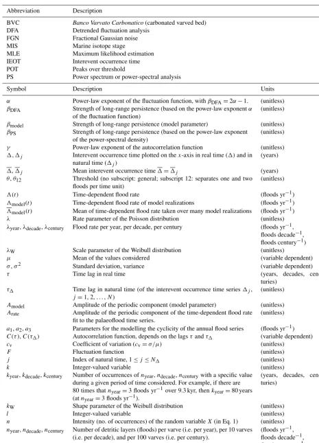
Table 1.Abbreviations and notation.

Abbreviation Description

BVC Banco Varvato Carbonatico(carbonated varved bed)

DFA Detrended fluctuation analysis

FGN Fractional Gaussian noise

MIS Marine isotope stage

MLE Maximum likelihood estimation

IEOT Interevent occurrence time

POT Peaks over threshold

PS Power spectrum or power-spectral analysis

Symbol Description Units

α Power-law exponent of the fluctuation function, withβDFA=2α−1. (unitless)

βDFA Strength of long-range persistence (based on the power-law exponentα

of the fluctuation function)

(unitless)

βmodel Strength of long-range persistence (model parameter) (unitless)

βPS Strength of long-range persistence (based on the power-law exponent

of the power-spectral density)

(unitless)

γ Power-law exponent of the autocorrelation function (unitless)

1, 1j Interevent occurrence time plotted on thex-axis in real time (1)and in

natural time (1j)

(years)

1,1j Mean interevent occurrence time1=1j (years)

θ,θ12 Threshold (no subscript: general; subscript 12: separates one and two

floods per time unit)

(unitless)

3(t ) Time-dependent flood rate (floods yr−1)

3model(t) Time-dependent flood rate of model realizations (floods yr−1)

3model(t ) Mean of time-dependent flood rate taken over many model realizations (floods yr−1)

λ Rate parameter of the Poisson distribution (unitless)

λyear,λdecade,λcentury Flood rate per year, per decade, per century (floods yr−1, floods decade−1, floods century−1)

λW Scale parameter of the Weibull distribution (unitless)

µ Mean of the values considered (variable dependent)

σ,σ2 Standard deviation, variance (variable dependent)

τ Time lag in real time (years, decades,

cen-turies)

τ1 Time lag in natural time (of the interevent occurrence time series1j,

j=1, 2, . . . ,N)

(unitless)

Amodel Amplitude of the periodic component (model parameter) (unitless)

Arate Amplitude of the periodic component of the time-dependent flood rate

fit to the palaeoflood time series.

(unitless)

a1,a2,a3 Parameters for the modelling the cyclicity of the annual flood series (floods yr−1)

C(τ ),C(τ1) Autocorrelation function, depends on the lagsτandτ1 (variable dependent)

cv Coefficient of variation (cv=σ/µ) (unitless)

F Fluctuation function (unitless)

j Index of natural time, 1≤j≤N1 (unitless)

k Integer-valued variable (unitless)

kyear,kdecade,kcentury Number of occurrences ofnyear,ndecade,ncenturywith a specific value during a given period of time considered. For example, if there are 80 times thatnyear=3 floods yr−1over 9.3 kyr, thenkyear=80 years (atnyear=3 floods yr−1).

(years, decades, cen-turies)

kW Shape parameter of the Weibull distribution (unitless)

l Integer-valued variable (unitless)

n Intensity (no. of occurrences) of the random variableX(in Eq. 1) (unitless)

nyear,ndecade,ncentury Number of detritic layers (floods) per varve (i.e. per year), per 10 varves (i.e. per decade), and per 100 varves (i.e. per century).

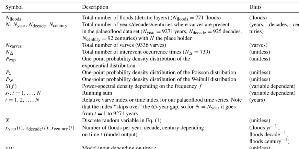
Table 1.Continued.

Symbol Description Units

Nfloods Total number of floods (detritic layers) (Nfloods=771 floods) (floods)

N,Nyear,Ndecade,Ncentury Total number of years/decades/centuries where varves are present

in the palaeoflood data set (Nyear=9271 years,Ndecade=925 decades,

Ncentury=92 centuries) withNthe place holder

(years, decades, cen-turies)

Nvarves Total number of varves (9336 varves) (varves)

N1 Total number of interevent occurrence times (N1=739) (unitless)

Pexp One-point probability density distribution of the

exponential distribution

(unitless)

Pλ One-point probability density distribution of the Poisson distribution (unitless)

PW One-point probability density distribution of the Weibull distribution (unitless)

S(f ) Power-spectral density depending on the frequencyf (variable dependent)

st,t=1, . . . ,N Running sum (variable dependent)

t=1, 2, . . . ,N Relative varve index or time index for our palaeoflood time series. Note

that the index “skips over” the 65-year gap, so forN=Nyearit goes

fromt=1 to 9271 years.

(years)

X Discrete random variable in Eq. (1) (unitless)

xyear(t ),xdecade(t ),xcentury(t ) Number of floods per year, decade, century depending

on timet(model output)

(floods yr−1, floods decade−1, floods century−1)

y(t ) Model input depending on timet (unitless)

The timings of the considered 771 palaeoflood events are transformed into three event series (Fig. 3), the number of floods (detrital layers) per year (nyear), per decade (ndecade),

and per century (ncentury), over the 9271 years of

palae-oflood data (over a 9336-year record). These three data sets are integer-valued time series which contain Nyear=9271,

Ndecade=925, and Ncentury=92 data points, and will

pro-vide the basis for our time series analyses in Sect. 4. In these three palaeoflood time series (Fig. 3) which represent our data, we observe that there are time periods with little fluc-tuation of the number of floods per century (i.e. the 24th to 18th centuries with values over the range 10–16 floods century−1). However, we also see sudden transitions from many to a few floods (as from 24 to 4 floods century−1from the 39th to 38th centuries) as well as from a few to many floods (as from 7 to 25 floods century−1 from the 46th to 45th centuries).

The histograms of these data are also given in Fig. 3, on the far right of each time series. The number of years (kyear) with no floods (nyear=0 floods yr−1) is

kyear=8530 years (92.0 % of the record). Similarly, for

nyear=1, 2, 3 floods yr−1, the number of years

(respec-tively) with those values arekyear=712 (7.7 %), 28 (0.3 %),

and 1 (0.01 %) years. For Nyear=9271 years examined,

there are 741 years which have 1 to 3 floods (detrital lay-ers), a total of 771 floods. We will revisit these values in Sect. 4.1. The data cover Ndecade=925 non-overlapping

decades (because of the 65-year gap, 8 of the decades within the 9336 years are disrupted). The number of decades (kdecade) with no floods (ndecade=0 floods decade−1) is

kdecade=453 decades (49.0 % of the record). Similarly, for

ndecade=1, 2, 3 floods decade−1,kdecade=283 (30.6 %), 123

(13.3 %), and 43 (4.6 %) decades. For 4≤ndecade≤8 floods

decade−1, kdecade=23 (2.5 %) decades. No decades have

ndecade> 8 floods decade−1. If we consider the data on the

century resolution, we have Ncentury=92 non-overlapping

centuries, as the 65-year gap falls completely within 1 cen-tury. The number of centuries (kcentury) with no floods

(ncentury=0 floods century−1)iskcentury=1 century (1 % of

the record). For 1≤ncentury≤5 and 6≤ncentury≤10 floods

century−1, kcentury=26 and 35 centuries (28 and 38 % of

the record) respectively. Forncentury > 10 floods century−1,

kcentury then decreases (Fig. 3), with a maximum value of

ncentury=31 floods century−1 which is reached once (i.e.

kcentury=1 century).

0 1 2 3 4

(a.1)

8100 8120 8140 8160 8180 0

1 2 3

4 (a.2) _{= 3 yr}

= 26 yr

nyear

[

floods

yr

−

1 ]

t [yr]

= 52 yr

0 2000 4000 6000 8000

1 10

100 (b)

Int

e

re

ve

nt

o

cc

u

rr

e

n

ce

ti

m

e

,

[yr

]

Relative age (varve index), t [yr]

0 100 200 300 400 500 600 700

1 10 100

(c)

Int

e

re

ve

nt

o

cc

u

rr

e

n

ce

ti

m

e

,

[yr

]

Natural time (detrital varve index), j

F

loo

ds

per

yea

r,

nyear

[f

lo

od

s

yr

]

Figure 4.Data series of detrital layers (floods) and interevent occurrence times (IEOTs) from the Piànico–Sèllere, Italy, palaeoflood sequence.

(a)In panel(a.1)are shown the number of detrital layers (floods) per varve,nyear, given as a function of varve indext=1 to 9336 years

(blue dots – data available at Mangili et al., 2017) as shown in Fig. 3. In panel(a.2)a 100-year portion of (A.1) (fromt=8090 to 8190 years)

is expanded with an illustration of 4 flood years that have detrital layers (floods) in them, and the interevent occurrence times1between

them. These 4 flood years, each withnyear≥1 flood in them, appear as yellow symbols in all panels. (b) Interevent occurrence times,1,

temporally located (i.e. as a function of the relative age) when they occurred. (c) Interevent occurrence times,1j, plotted as a function of

“natural” time, where each1is no longer represented temporally when it occurs, but rather successively one after another,j=1, 2, 3, . . . ,

741; interevent occurrence times of1j=0 are not shown. The detrital varve indexj includes only those years (varves) where there are

nyear≥1 floods yr−1(i.e. at least one detrital layer in that year).

can identify when a flood is thought to have occurred, this does not preclude the possibility that other floods occurred but were not identified as a detrital layer. We do acknowledge research (e.g. Corella et al., 2014; Schillereff et al., 2014) where the type and thickness of detritus in Holocene varves are used to make interpretations of the strength of a hydro-meteorological event; however, due to the age of our sedi-ments this sort of analysis of event magnitude was not possi-ble here. In this paper, we therefore focus on just the tempo-ral attributes of the 771 floods themselves over this 9336-year period in the Pleistocene. See data availability for access to the palaeoflood database.

Section but present in the Wall Section. Overall, this repre-sented a total of 889 out of 896 varves (99.2 %) in common between the two outcrops, which means that if we extend their results to the other 90 % of the outcrop, some uncer-tainty might exist, with up to 1 % of the varves “missing” in time, which should have a very small impact on the relative timing of floods discussed in this paper.

The analyses in this paper will concentrate on the fluctua-tions in flood frequency over time (i.e. the number of floods per year and per decade), examining the temporal correla-tions,clustering, andcyclicityof the flood frequencies. Be-fore proceeding to the analyses of these time series, we pro-vide next (Sect. 3) the definitions and methods used in sub-sequent sections.

3 Definitions and methods for the analysis of event series

Both correlations and clustering were introduced in Sect. 1. Here we provide more in-depth definitions and explanations of clustering and correlation methods that will be used in ex-amining our palaeoflood time series. In Sect. 3.1, we intro-duce interevent occurrence times (IEOTs). Then, in Sect. 3.2, Poisson processes, a model for correlated and non-clustered time series. Section 3.3 describes the Weibull dis-tribution (in the context of IEOTs) as an indicator of clus-tering. Section 3.4 introduces autocorrelation as a method to quantify short-range and long-range correlations in a given time series. In Sect. 3.5, we describe power-spectral analysis and detrended fluctuation analysis as methods for quantify-ing long-range correlations. Finally, in Sect. 3.6 we briefly introduce fractional noises.

3.1 Interevent occurrence times

In this paper, we will consider the number of palaeofloods per year, decade, and century as event series in time. As indi-cators of clustering and/or correlations (or lack thereof), we will apply statistical methods to the event magnitudes (i.e. the number of floods per year, decade, or century). We will also consider the time intervals between successive events, i.e. the interevent occurrence times (IEOTs) which we intro-duce here. We will later use the statistical distribution of the IEOTs as an indicator of clustering (or lack of) in the original time series.

We introduce IEOTs in the context of our yearly palae-oflood time series (top panel of Fig. 3) where, as previ-ously, t is the relative age in years in our time series and nyear is the number of floods per year. First, we define a

flood year to be any year t with at least one flood in it, i.e. nyear(t)≥1 flood yr−1. Second, we define IEOT as the

time interval 1 between successive years that have one or more floods, i.e. more formally, nyear(t)≥1 flood yr−1and

nyear(t +1)≥1 flood yr−1, but for all years in-between,

nyear(t+l)=0 floods yr−1forl=1, 2, . . . ,1−1.

In Fig. 4a we illustrate finding the IEOTs: we present the number of detrital layers per year (Fig. 4a.1, which is the same as the top panel in Fig. 3) with as inset (Fig. 4a.2) an ex-ample of four detrital layers with IEOTs of1=52, 3, and 26 years. In Fig. 4b we give all the1as a function of relative age t for the entire palaeoflood data set. The values of1range from 1 to 125 years (with quartiles of 25 %: 3 years, 50 %: 7 years, and 75 %: 15 years) and a mean1=12.5 years. We then use a subscriptj to indicate successive IEOTs,1j,

which we plot using “natural” time, in other words where each1is no longer represented temporally when it occurs, but rather successively one after another,j=1, 2, 3, . . . ,N1,

with the total number of natural time intervalsN1=739 (we

discard thej value corresponding to the gap). In Fig. 4c we plot the same1from Fig. 4b, but now as a function of the detrital varve index (natural time),j=1, 2, 3, . . . ,N1.

The use of natural time (i.e. the time between all events is “equal” in natural time) to represent unequally spaced events in time series has been mainly used to examine seismic-related time series (e.g. Uyeda et al., 2009; Rundle et al., 2012), but has found use in a variety of other disciplines ranging from biology and environmental sciences to cardi-ology (see Varotsos et al., 2011, for a review of its use in various disciplines).

3.2 Poisson process as a model for an uncorrelated non-clustered time series

The standard example of an event series that is uncorrelated in time, non-clustered, and stationary in time is the realiza-tion of a Poisson process. In later analyses (Sect. 4.1) we will compare the statistical distribution of the magnitudes in our three palaeoflood time series (Fig. 3) to those of a Poisson process, thus inferring the lack of correlations and cluster-ing (if a Poisson process) or the presence of correlations or clustering (if not a Poisson process). If a real-world process (e.g. flooding) by which a time series results is assumed to be Poissonian, then many synthetic realizations of that Poisson process can be created, and their statistical properties con-fronted with those of the observed “real-world” time series. Poisson processes have been found in some cases to model the temporal occurrence of floods (e.g. Kirby, 1969; Todor-ovic and Zelenhasic, 1970) and in other cases to not be an appropriate model (e.g. Mudelsee et al., 2004, who showed that the winter floods of the Elbe River from 1500 to 2000 cannot be modelled by a stationary Poisson process).

For a time series to be considered a realization of a Poisson process, the following must be true (Cox and Lewis, 1978):

i. the time series elements are non-negative integers; ii. the time series considered is stochastic (i.e. has no

iii. the one-point probability distribution of the time series elements follows a Poisson distribution, that is, a posi-tive integer-valued random variableX, whose probabil-ity densitiesPλare defined as (Cox and Lewis, 1978)

Pλ(X=n)=

λn

n!exp(−λ) , n=1,2,3, . . . (1) where “!” means factorial, exp is the exponential func-tion,λis the rate parameter withλ> 0, andnis the in-tensity (number of occurrences) of the “random” vari-able per given time unit (e.g. hour, year, decade, cen-tury). The rate parameter λ is a physical quantity and thus has units (time unit)−1_{, but the Poisson process as}

given in Eq. (1) is a mathematical model andPλ does

not have units.

iv. the times between successive events (interevent occur-rence times, IEOTs) are independent in time (i.e. there is no correlation between one IEOT and others, so events occur independently of one another);

v. the one-point probability distributionP of the IEOTs1 is exponential with

Pexp(1)=λexp(−λ1) , 1≥0 (2)

with the same rate parameter λ as in Eq. (1) and the time unit of the original time series being small enough that almost all time units have just no or one event (i.e. λ1).

The Poisson process as defined in Eq. (1) does not lead to any temporal clustering. The one-point probability distribu-tion for the Poisson process for 0< λ≤1 had no mode, and forλ >1 it has a defined mode.

3.3 Weibull distribution of IEOTs as an indicator of clustering

If the1j (the IEOTs), in addition to not being exponentially

distributed, are Weibull distributed, this is taken as an indi-cator of clustering of the original time series (Bunde et al., 2005; Witt et al., 2010). The two-parameter Weibull proba-bility distribution (Weibull, 1951) is a standard waiting time distribution, i.e. frequently used for modelling the time inter-vals between successive events (Cox and Lewis, 1978). The continuous (vs. discrete, as in Eq. (1) for the Poisson distribu-tion) two-parameter Weibull probability distribution is given by (Weibull, 1951)

PW(1)=

kW

λW

₁

λW

kW−1

exp

"

−

₁

λW

kW#

, 1≥0 (3)

where the two parameters areλWfor scale andkWfor shape,

and1is any real number ≥0. When the shape parameter kW=1.0, the two-parameter continuous Weibull distribution

(Eq. 3) turns into PW(1)=

1 λW

exp

−1

λW

, 1≥0, (4)

that is, the exponential distribution which describes the IEOT distribution of a Poisson process with a parameterλ=1/λW

(see Eq. 1).

For shape parameters 0.0 <kW< 1.0, the two-parameter

Weibull distribution (Eq. 3) is heavy-tailed (i.e. asymptoti-cally scale invariant) with a tail parameter of (1−kW), which

means that the probability density for very large values1in Eq. (3) scales with a power law with the tail parameter as power-law exponent.

3.4 Autocorrelation as a method for quantifying temporal (short-range and long-range) correlations There are a variety of methods that can be used to explore and quantify temporal correlations both in observed time se-ries and realizations of a modelling process. As discussed in Sect. 1, correlations (persistence) have been studied in many environmental time series. Measures for correlations quan-tify the statistical dependence between variables, and in par-ticular, measures fortemporal correlations describe the in-tensity of this relation between time series elements with a fixed temporal distance. To quantify the strength of corre-lations, we use autocorrelation analysis applied to the time series of number of floods per year (nyear), decade (ndecade),

and century (ncentury)(Fig. 3). The autocorrelation function

C(e.g. Priestley, 1982) for the number of floods is defined as

C (τ )= 1 N σ2_(n)

N−τ

X

j=1

nj−n nj+τ−n (5)

wherenj is a time series of the number of floods per year

(decade, century) with j =1,2, . . . , N, with N=Nyear,

Ndecadeor Ncentury (i.e. the total number of years, decades,

a given year, on average,τ years later will be followed by a very few number of floods (compared to the mean number of floods per year overall).

If the correlations are essentially linear and thus can be de-scribed by the autocorrelation function, two types of correla-tions can be considered: (i) short-range correlacorrela-tions (Priest-ley, 1982; Box et al., 2013) and (ii) long-range correlations (e.g. Taqqu and Samorodnitsky; 1992; Beran, 1994; Mala-mud and Turcotte, 1999).

Short-range correlations are characterized by a decay of the autocorrelation functionC(τ )(Eq. 5) that is bounded by an exponential decay for large lags,τ:

|C (τ )| ≤γ0exp(−γ τ ) , τ > τ0, (6)

whereτ0,γ0, andγ are non-negative constants. In

particu-lar, this definition applies for time series with a finite correla-tion length (C(τ )=0 forτ>τ0). Statistical models for

short-range correlated time series include autoregressive (AR) and moving average (MA) processes (Priestley, 1982).

In contrast to short-range correlated time series, long-range correlated time series approach a power-law decay of the autocorrelation functionC(τ )(Eq. 5) for large lagsτ: C (τ )∼τ−(1−β),0.0<β<1.0. (7) The parameter β (0.0<β<1.0) is the strength of the long-range correlations. The autocorrelation function has two lim-iting values: β=0.0 (which represents short-range persis-tence between the time series elements) andβ=1.0 (pink or 1/fnoise). Koutsoyiannis and Montanari (2007) have shown that the statistical uncertainty of the mean value of (hydrolog-ical) time series is increased in the presence of correlations, and in particular long-range correlations.

3.5 Power-spectral analysis and detrended fluctuation analysis (DFA) for quantifying long-range

correlations

In the last section, we used the autocorrelation function as one method to quantify long-range (and short-range) cor-relations. Here we describe two more methods for quanti-fying long-range correlations: power-spectral analysis and detrended fluctuation analysis. We focus on long-range (vs. short-range) correlations as these form the main part of our analyses and modelling in later sections. These two meth-ods are both more robust than autocorrelation in quantifying long-range correlations (Witt and Malamud, 2013).

Long-range correlations are reflected by a scaling of the power-spectral density S (square of the modulus of the Fourier coefficients appropriately normalized) with fre-quencyf. The power-spectral densitySexhibits a power-law scaling such that (Taqqu and Samorodnitsky, 1992; Beran, 1994)

S (f )∼f−β, (8)

wheref is the frequency and the relationship holds (for long-range persistence) over allβ (Pelletier and Turcotte, 1999; Witt and Malamud, 2013). Positive exponents (β> 0.0) in Eq. (8) represent positive (long-range) persistence and neg-ative ones (β< 0.0) anti-persistence. The specific case of β=0.0 corresponds to an uncorrelated time series (e.g. a white noise), and a value ofβ=1.0 is known also as a 1/f or pink noise (Mandelbrot and van Ness, 1968; Bak et al., 1987). Some examples of these long-range persistent time series are given in the next Sect. 3.6. In this paper, to avoid confusion with other estimators (e.g. DFA; see next), we will indicate the measurement of the strength of long-range per-sistence by power-spectral analysis using the notationβPS.

Another common method for quantifying long-range cor-relations is detrended fluctuation analysis (DFA) (e.g. Peng et al., 1994; Kantelhardt et al., 2001). Here, the scaling prop-erties of long-range correlated time series are quantified in terms of the fluctuation function. In this paper the number of floods per year, decade, or century can be analysed by DFA; we call these time series herext,t=1, . . . ,N. The

fluctua-tion funcfluctua-tion is based on the running sums (or profile) of the considered time seriesxt,t=1, . . . ,N:

st = t

X

i=1

xi. (9)

This time series of the running sumsst,t=1, . . . ,Nis then

split up into non-overlapping segments of lengthl. For the kth segment of the running sums,sk,i,i=1, . . . ,l, the

fluc-tuation is determined as the variance of the difference of this segment and its best-fitting polynomial trendtk,i,i=1, . . . ,

l(with the polynomial orderk, usually between 1 and 4),

F2(k, l)=1 l

l

X

i=1

sk,i−tk,i2. (10)

The fluctuation of the time series is the mean of the fluctua-tion of the segments:

F2(l)=DF2(k, l)E

k, (11)

whereh i_k is the mean value taken over all fluctuations of lengthksegments. If the underlying time seriesxt,t=1, . . . ,

N has long-range correlations, then the fluctuation function F (l)exposes for long segment lengthsla power-law scaling and will scale as (Peng et al., 1992)

F (l)∼lα. (12)

- 20

2

4

P i n k n o i s e

W h i t e n o i s e

 = 0 . 0

F

ra

c

ti

o

n

a

l n

o

is

e

,

xt - 2

0

2

4  = 0 . 2

- 20

2

4 _{ = 0 . 4}

- 20

2

4

 = 0 . 8  = 0 . 6

- 20

2

4

 = 1 . 0

0 1 2 8 2 5 6 3 8 4 5 1 2

- 20

2

4

Time, t

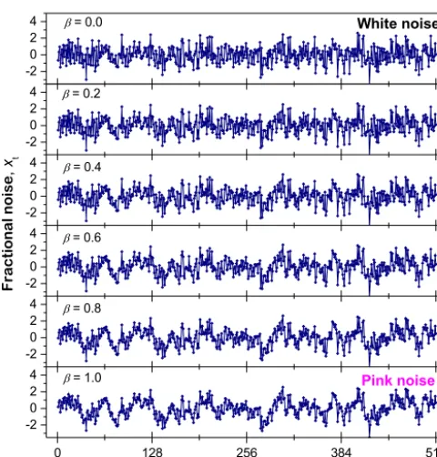
Figure 5. Examples of synthetic fractional Gaussian noises with

different modelled strengths of long-range persistence, 0.0≤β≤

1.0. The presented synthetic data series (unitless in magnitude and

time), which have 512 elements each, are normalized to have a mean of 0 and a standard deviation of 1, and were created by Fourier filtering (see Appendices 1 and 2 in Witt and Malamud, 2013, for further details).

the notation βDFA (to indicate the use of DFA) based on

βDFA=2α−1.

For Eqs. (7) (autocorrelation analysis), (5) (power-spectral analysis), and (9) (DFA), in each case we have an inverse power-law decay with increasing temporal scales (lag, fre-quency, temporal segment length), which defines a self-affine time series (the time series is statistically self-similar when comparing different temporal scales) (Mandelbrot and Van Ness, 1968). If the power-law exponent held over “all” tem-poral scales (which it rarely does), then the correlation length (the largest lag or temporal scale at which there are still sta-tistical correlations in the time series) would be infinite. One potential significance of this “infinite” correlation length is that “all” values are statistically correlated with one another in the time series. A second significance is that the time series can be explained as a stochastic fractal (Malamud and Tur-cotte, 1998). In the case of our palaeoflood series this means potentially that the flood timings are organized in time as the points of a Cantor dust (see Ott, 1993, for a discussion of Cantor sets).

Extensive details about power-spectral analysis, DFA, and software written in R (R Core Team, 2013) for performing time series analysis using these techniques are given in the review paper by Witt and Malamud (2013). This latter study

also investigates biases of both techniques which typically occur when they are applied to time series that have a one-point probability distribution that is strongly non-Gaussian and/or the time series has very few values (e.g. just a few thousand data).

3.6 Fractional noises as examples of long-range correlated time series

Fractional noises are standard examples of long-range corre-lated time series (Malamud and Turcotte, 1999; Mandelbrot, 1999), which we will use here to help us model long-range persistent characteristics of our palaeoflood time series. Ex-amples of six fractional noises are shown in Fig. 5, with the strength of long-range persistence ranging fromβ=0.0 (a white noise) toβ=1.0 (a pink noise), in 0.2 increments. In the white noise in Fig. 5, the values are uncorrelated with each other, and as we increase the strength of long-range per-sistence, the values, although drawn from the same under-lying probability distribution, become more correlated with one another (and their clustering increases).

4 Results of statistical metrics, clustering, correlations, and cyclicity of the palaeoflood sequence

In this section, we first statistically analyse the 771 timings of palaeofloods in terms of their elementary metrics of the number of palaeofloods per year, decade, and century com-pared to a Poisson process (Sect. 4.1). We then examine the probability of IEOTs compared to a Weibull distribution as a potential indicator of clustering (Sect. 4.2). Next, we use autocorrelation of the palaeoflood time series to charac-terize the temporal correlations (Sect. 4.3) and autocorrela-tion of the IEOTs as another potential indicator of clustering (Sect. 4.4). We then characterize the temporal correlations of the time series using detrended fluctuation analysis and power-spectral analysis (Sect. 4.5). Finally, we characterize the cyclicity of the palaeoflood time series using a sinusoidal model (Sect. 4.6). As the techniques we used are designed for time series with a continuous one-point probability distribu-tion (e.g. Gaussian, log-normal, or Levy distribudistribu-tion) vs. the integer values that are found in our palaeoflood time series, we throughout also show the statistical significance of our findings.

4.1 Number of palaeofloods per year, decade, and century, compared to a Poisson process

Pois-0 1 2 3 4 5 6 7 8 0

200 400

600 Decadal data Poisson model

Floods per decade, n_decade

D

ecades

,

kdeca

de

0 50 100 150 200 10-1

100 Decadal

97.5 % of Poisson model

Time lag, [yr]

−0.33

0 1 2 3

0 5000 10000

Yearly data Poisson model

Y

ears

,

kyear

0 50 100 150 200 10-2

10-1 100 Yearly

(b)

97.5 % of Poisson model Floods per year, n_year

A

ut

oco

rr

el

at

ion

funct

ion,

C

0 25 50 75

(a)

0 5 101520253035 Floods per century, n_century

Centennial data Poisson model

C

enturi

es

,

kcentury

0 100 200

10-1

100 Centennial

97.5 % of Poisson model

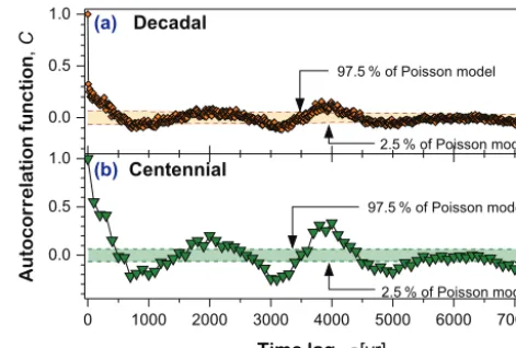
Figure 6.Histograms and autocorrelation of the palaeoflood time series with the corresponding Poisson model.(a)Histogram (also shown in

Fig. 3) of the number of floods per year (blue bars), decade (orange bars), and century (green bars), with each compared to the Poisson model with respective rate parametersλyear=0.083 floods yr−1,λdecade=0.83 floods decade−1, andλcentury=8.3 floods century−1. Diamonds

represent the mean Poisson model value and the error bars the standard deviation over 100 realizations.(b)Autocorrelation function (ACF)

(Eq. 5) of the number of floods per year (blue squares), decade (orange squares), and century (green squares). Also shown for the ACF of the number of floods per decade is the best-fitting power-law model to the ACF (black dotted line) (Eq. 13). Also shown are the 97.5th percentile,

i.e. the upper bound of the 95 % confidence interval of the ACF (for lagsτ >0) of an uncorrelated signal with the same one-point probability

distribution (i.e. realization of a Poisson model).

0 25 50 75 100 125

10-1

100

101

102 _{Observed data}

Poisson model Weibull distribution

Interevent occurrence time, [yr]

Fr

equen

cy

den

si

ty,

f

(

)

[yr

1 ]

(a)

1 10

10-1

100

Upper limit of the 95 % confidence interval for uncorrelated IEOTs

C(IEOT between flood years)

Power-law model

Time lag (in natural time), ∆

Au

to

co

rre

la

tion

fun

ct

ion

,

C (b)

∆

∆

∆

Figure 7. Frequency-size and autocorrelation analysis of the interevent occurrence times (IEOTs) and comparison to the Poisson model.

(a)Frequency density of the IEOTs between the flood years given as a function of IEOTs in years (pink vertical bars, semi-logarithmic

scale), the corresponding best-fit Poisson model (grey diamonds) (Eq. 2) which was considered in Fig. 6, and the best-fit Weibull distribution

(black diamonds) (Eq. 3), both with 95 % confidence intervals. (b) Autocorrelation function (Eq. 5) of the IEOTs between flood years

(those years withn≥1 flood). Also given is the best-fitting power-law model (dashed black line) (Eq. 14) and the upper limit of the 95 %

significance for the autocorrelation function of a non-correlated time series with the same one-point probability distribution (horizontal dotted line, pink).

son process with a constant rate parameter to create model time series of flood events per year, decade, and century (i.e. similar to the palaeoflood time series shown in Fig. 3). We will see below that the resultant model realizations will be stationary, uncorrelated in time, and non-clustered, and then

show in subsequent sections that this modelling is inappro-priate for our palaeoflood time series.

We first interpret the numbernin Eq. (1) as the number of detrital layers per varve (nyear, floods yr−1). The rate

num-ber of events per year (i.e. per varve) isnyear=λyearand the

variance of the number of events isσ2 nyear=λyear. This

equation holds only mathematically but not physically, i.e. it holds for the numbers but not for the units. The probability in Eq. (1) is not time dependent, and rather only depends on (if we take our unit of time to be 1 year) the probability of nyear=1 flood yr−1,nyear=2 floods yr−1, etc., and not the

relative temporal spacing of the floods in time. To model the series of the number of flood events per year in the 9.3 kyr Piànico–Sèllere palaeoflood time series, we use a (constant) rate parameter of λ=0.083 floods yr−1 that is the mean number of detrital layers per varve, i.e. (771 floods)/(9271 years)=0.083 floods yr−1, where we discard the 65-year gap for the total number of years considered.

As discussed in Sect. 3.2, another consequence of consid-ering the number of floods per year as a Poisson process is that the time interval1between two successive events (i.e. the IEOTs between two successive floods) follows an expo-nential one-point probability distribution P for very small time units (Eq. 2) with rate parameter λ. Now, the relative ordering between single floods is taken into account. For ex-ample, if in a given decade we have three varves, each with one flood, Eq. (2) will be different if the 3 years with floods are in years 1, 2, and 3 (11=12=1 year, 13≥8 years

because the fourth flood will be in a subsequent decade) vs. one flood each in years 1, 5, and 9 of the decade (i.e. 11=12=4 years,13≥2 years). Note that the time

inter-val1can have non-integer values, for instance if two or more events (floods) occur in a single time unit (within 1 year).

For our palaeoflood time series (Fig. 3), we now consider whether the histograms (horizontal bars on the right-hand side of Fig. 3) of the observed number of years, decades, and centuries with a given number of floods per year, decade, and century follow Poisson distributions. For each palae-oflood time series, we create a Poisson model which con-sists of 100 realizations of a Poisson process, each realiza-tion with 9271, 927, and 92 (respectively, for year, decade, and century) time series elements and with rate param-eters λ=λyear=0.083 floods yr−1 =λdecade=0.83 floods

decade−1=λcentury=8.3 floods century−1 (the

measure-ments values are different as well as the units; the differences cancel out because of multiplication of measurement values and units). We discard the 65-year gap for the purposes of this model. Each realization therefore has values that are un-correlated in time and follow a Poisson distribution (Eq. 1). Many common software programs (e.g. Excel, R, Matlab) are able to easily generate such realizations.

We give the results of our Poisson model for each re-spective time resolution (year, decade, century) in Fig. 6a as diamonds (mean of the 100 realizations) ± error bars (standard deviation of the 100 realizations). We find that for the yearly data, the number of years observed (kyear)

with a given number of floods per year, nyear=0, 1, 2, 3

floods yr−1, follows closely the number of years given by the Poisson model. For example, returning to the values given

above, the number of years withnyear=0, 1, 2, 3 floods yr−1

is observed to be kyear=8530, 712, 28, and 1 years

(re-spectively), and with the Poisson modelkyear=8531±26,

709±25, 30±5, and 1±1 years (mean±standard devia-tion) (respectively). In contrast, for both the decadal and centennial data, the observed data set contains decades and centuries with many fewer or greater floods compared to the model data (see Fig. 6a). For example, the number of decades withndecade=0, 1, 2 floods decade−1 is observed

to be kdecade=453, 283, and 123 decades (respectively),

with the Poisson model givingkdecade=406±15, 338±13,

and 140±11 decades (mean±standard deviation) (respec-tively).

We therefore conclude that at the yearly scale the observed data follow a Poisson process, but at the decadal and centen-nial scales, the time series cannot be modelled as a Poisson process. In subsequent sections we will explore whether clus-tering, correlations, or both are responsible for this.

4.2 Probability of interevent occurrence times (IEOTs) compared to a Weibull distribution as a potential indicator of clustering

Here, we analyse the one-point probability distributions of the interevent occurrence times (IEOTs) (Sect. 3.1). As dis-cussed in Sect. 3.2, a realization of a Poisson process is characterized by “events” that are uncorrelated with one an-other and the1j have an exponential distribution (Eq. 2).

Conversely, it means that if the 1j (the IEOTs) are

non-exponentially distributed, the process is non-Poisson. In Fig. 7a, we give the frequency density of1(the one IEOT that includes the sediment gap is excluded) of the flood record along with an exponential distribution which repre-sents the interevent occurrence times of events in a Poisson process. The distribution of the IEOTs has a higher number of both short and long time intervals compared to an ex-ponential distribution. This observation is supported by sta-tistical hypothesis testing where an Anderson–Darling test (Anderson and Darling, 1952) was adjusted to integer val-ues of the IEOT distribution (using a method described in Choulakian et al., 1994; Arnold and Emerson, 2011), and the test rejected the null hypothesis that this distribution can be explained as the result of a Poisson process (p-value < 0.002).

We have shown above that our data are not a Poisson pro-cess, and now wish to further characterize the distribution of the IEOT. For the palaeoflood IEOTs, we use a maximum-likelihood estimation (MLE) and assume a two-parameter Weibull distribution (Eq. 3 and discussed in Sect. 3.3). We find (see Fig. 7a) a best-fit shape parameter for the Weibull distribution ofkW=0.91±0.024, where the error bars

val-ues. Therefore, we use benchmarks (500 realizations of a Weibull distributed model for random numbers) for fitting Weibull distributions to integer-valued data. We find that the MLE estimator tends to over-fit the shape parameter by 0.12, i.e. we can correct our estimate of the shape parameter to kW=0.79±0.024.

4.3 Autocorrelation of palaeoflood sequences to quantify correlations

We now use the autocorrelation function (ACF) discussed in Sect. 3.4 and apply it to our palaeoflood sequence as a po-tential indicator of correlations. In our analyses of the palae-oflood sequence, only pairs of years, decades, or centuries nj, nj+τwhich do not contain the 65-year gap in the

9336-year sequence of floods (detrital layers) are considered. The autocorrelation function (Eq. 5) applied to the time series of the number of floods per year, decade, and century is given as correlograms in Fig. 6b (squares). This correlogram of the yearly floods shows significant positive correlations with a decaying trend and no obvious periodic components for lags of 1≤τ ≤200 years. Due to the strongly fluctuating be-haviour of the annual data’s correlogram (squares) in Fig. 6b it is difficult to determine the functional form of the decay, i.e. to decide whether the decay is exponential (thin tailed, short-range persistent) or approaching a power law (heavy tailed, long-range persistent). Therefore, we apply the auto-correlation function to the time series of the number of floods per decade (with respect to non-overlapping 10-year time in-tervals) and find (Fig. 6b) a power-law behaviour

C (τ )∼τ−γACF_{, τ >0 (13)}

with a power-law exponent for the decadal time series of γACF=0.34±0.04 (fitted for lags 1≤τ≤20 decade,

which is equivalent to 10≤τ≤200 years) with uncertainties ±1 standard error of the exponent. Comparing to Eq. (7), γACF=(1−βACF), givingβACF=0.66 ±0.04. We will

re-turn to this power-law model (Eq. 13) in Sects. 4.5 and 5.2. We conclude that for the floods per decade time series, when using the autocorrelation function, the data exhibit long-range correlations over the long-range 10≤τ ≤200 years.

The time series of the number of floods per century con-tains only 92 data points. We therefore have calculated the autocorrelation functionC only for lagsτ=1 century and τ =2 century as graphically presented in Fig. 6b. Based on this figure, we see significant positive correlations and thus confirm the results found for the temporal correlations of the number of floods per year and decade. Due to the very few lag values, however, we cannot discuss the functional shape of this autocorrelation function.

We conclude that the three considered time series nyear,

ndecade, andncenturyhave positive autocorrelations for lags of

τ< 200 years. For the number of floods per decade,ndecade,

we find indications of a power-law shape of the autocorrela-tion funcautocorrela-tion which indicates long-range persistence of the

time series over lags τ> 200 years. However, we will see later (Sect. 4.6) for lagsτ> 200 years that a power-law model cannot be conclusively fit, and thus over all lags, we cannot conclusively use ACF as a robust quantifier of long-range correlations.

4.4 Autocorrelation of interevent occurrence times (IEOTs) as a potential indicator of clustering Another indicator of clustering is positive temporal correla-tions of the IEOTs (Sect. 3.1). Such correlacorrela-tions are partic-ularly caused by a “lumping” of small (large) IEOTs which results in time intervals with an increased (decreased) flood rate which correspond to flood clusters (phases of little flood-ing activity). In Fig. 7b, we examine correlations (vs. cluster-ing) of the IEOTs by applying the autocorrelation function (Eq. 5) to the1j for the IEOTs. We find significant positive

correlations of the 1j for flood year lags 1≤τ1≤20 (no

units). This indicates that for the IEOT, small values of1j

tend to follow small ones, and large ones tend to follow large ones. Similar to Eq. (13), the correlogram (see Fig. 7b) of1j

exhibits a power-law behaviour C (τ1)∼τ

−γ1

1 , γ1>0 (14)

with a power-law exponent of γ1=0.45 ±0.14 (fit for

lags of 1≤τ1≤20 IEOTs, which is equivalent to 12.5≤

τ≤250 years). Power-law correlations for IEOTs are re-ported for a class of theoretical models by Bunde et al. (2003) and Eichner et al. (2007), who have studied peaks over thresholds of long-range correlated time series. We will ex-plore this in more detail below.

In summary, we have analysed the one-point probability distribution and the autocorrelation function of the IEOTs of the palaeofloods with respect to a time resolution of 1 year (i.e. we have not used time resolutions between palaeofloods that are sub-annual, such as 3 months). The distribution of the IEOTs can be well approximated by a Weibull distribution with a shape parameter ofkW=0.78. Therefore, the IEOTs

are more likely to be very short or very long temporal peri-ods compared to a random (uncorrelated) occurrence of the IEOTs, and therefore the palaeoflood time series is not a re-alization of a Poisson process. Furthermore, the IEOTs have positive temporal correlations. This is particularly caused by a clustering of the very high and very low IEOTs and thus by a temporal clustering of the floods. The autocorrelation function seems to follow a power-law behaviour.

4.5 Detrended fluctuation analysis (DFA) and

1 0 1 _{1 0} 2 1 0 0

1 0 1

P o w e r - l a w m o d e l , l 

 = 0 . 6 2 7 (_{D F A} = 0 . 2 5 )

F

lu

c

tu

a

ti

o

n

fu

n

c

ti

o

n

,

F

[(

10

y

r)

–

1 ]

Segment length,_{l [ 1 0 y r ]}

D F A 1 D F A 2 D F A 3 D F A 4

Figure 8.Detrended fluctuation analysis (DFA) of the 9271-year

Piànico–Sèllere, Italy, palaeoflood record: the fluctuation function

F for the number of floods per decade shown as a function of

the segment length l and for different orders of the detrending

(see the legend) on a double logarithmic scale. Segments contain-ing parts of or the entire gap were excluded. Also shown are the best-fitting power-law function (Eq. 12) for DFA3 and the

cor-responding power-law exponent αand its corresponding value of

βDFA=2α−1.

Sect. 3.5, both methods are more statistically robust than au-tocorrelation in quantifying long-range correlations. Meth-ods for quantifying long-range correlations have systematic and random errors in the resultant estimator for time se-ries with very asymmetric probability distributions and the finite size effects of the time series. The systematic error is how much the resultant estimator deviates from the un-derlying “correct” value, and random errors are the spread of the estimated quantity. Witt and Malamud (2013), us-ing 17 000 synthetic benchmark series, studied systemat-ically these two types of errors for power-spectral anal-ysis, DFA, and semivariogram analysis. ACF gives simi-lar results of robustness to semivariogram analysis due to the two methodologies being very similar. Witt and Mala-mud (2013) found that the systematic and random errors (bi-ases and standard errors) of DFA and PS analysis are signifi-cantly smaller (particularly for time series with non-Gaussian one-point probability distribution, and with very few val-ues in the time series) compared to semi-variogram anal-ysis, and both DFA and PS analysis are appropriate for a much broader range of long-range persistence strengths com-pared to semi-variogram analysis. We therefore only con-sider power-spectral analysis and DFA when concon-sidering the quantification of long-range correlations.

We start with our yearly flood record nyear which

con-tains 771 floods and extends over 9336 years. It has a heav-ily skewed one-point probability distribution with a

coeffi-cient of variation of cv=3.46. Witt and Malamud (2013)

showed that very asymmetric one-point probability distri-butions lead to a systematic underestimation of the persis-tence strength for both techniques. Due to the palaeoflood time series elements being integer valued and in a small range (0≤nyear≤4 floods yr−1), both techniques lead to

un-certain results. Therefore, we will not apply power-spectral analysis and DFA to the annual palaeoflood data set. But we will quantify long-range persistence of the decadal and centennial flood series, as the data are less heavily skewed (cv=1.30 and 0.77 respectively), and where there is a wider

range of integer values (0≤ndecade≤8 floods decade−1and

0≤ncentury≤31 floods century−1).

In Fig. 8 we show the results of the DFA analysis of ndecade. The fluctuation functions for different orders of

de-trending are shown on logarithmic axes. The almost lin-ear shape indicates power-law behaviour of the fluctuation function (see Eq. 12) for DFA3 and DFA4. DFA1 (DFA2) follows this linear shape just for segment lengths up to 70 (100) decades. We expect a slowly varying trend (a long-term cyclicity > 700 (1000) years) to cause this dependence on the type of detrending and will analyse it in more detail in Sect. 4.6. The power-law exponent for the decadal palae-oflood time series was estimated (for DFA3) asαDFA=0.62,

which corresponds to a strength of long-range persistence of βDFA=0.25. This is a weak strength of long-range

persis-tence. The third data set that counts the number of floods per century contains just 92 time series elements, which is not enough for a reliable DFA.

Power-spectral analysis for the decadal palaeoflood se-riesndecadeis shown in Fig. 9. Although the power-spectral

densityS has a lot of scatter, it is clearly oriented along a line in the log–log axes, and thus exposes power-law (self-affine) behaviour (see Eq. 8). The persistence strength (i.e. the magnitude of the law exponent of the power-spectral densityS) is estimated asβPS=0.39. This again

in-dicates a weak strength of long-range persistence. The cen-tennial palaeoflood series ncentury is not suited for

power-spectral analysis due to the short length ofNcentury=92

cen-turies.

We also see the hint of long-term periodic components superimposed onto the long-range persistence that is iden-tified using power-spectral analysis. In Fig. 9 are given three coloured lines that represent the 95th percentiles (95 %), de-scribed in detail in a later section (Sect. 5.1). What we ob-serve is that three values (large blue dots, outlined with a grey ellipse) are above the three 95 % lines (i.e. they are sig-nificant withp< 0.05) at a cyclicity of 1300 to 2300 years. Again, as for DFA, we will explore this long-term cyclicity (fluctuation) that appears to be superimposed onto the long-range persistent signal in the next subsection.