Mapping snow depth return levels: smooth spatial modeling versus station interpolation

www.hydrol-earth-syst-sci.net/14/2527/2010/ doi:10.5194/hess-14-2527-2010

© Author(s) 2010. CC Attribution 3.0 License.

Earth System

Sciences

Mapping snow depth return levels: smooth spatial modeling

versus station interpolation

J. Blanchet and M. Lehning

WSL Institute for Snow and Avalanche Research SLF, Davos, Switzerland

Received: 27 July 2010 – Published in Hydrol. Earth Syst. Sci. Discuss.: 25 August 2010 Revised: 30 November 2010 – Accepted: 3 December 2010 – Published: 13 December 2010

Abstract. For adequate risk management in mountainous

countries, hazard maps for extreme snow events are needed. This requires the computation of spatial estimates of return levels. In this article we use recent developments in extreme value theory and compare two main approaches for map-ping snow depth return levels from in situ measurements. The first one is based on the spatial interpolation of point-wise extremal distributions (the so-called Generalized Ex-treme Value distribution, GEV henceforth) computed at sta-tion locasta-tions. The second one is new and based on the direct estimation of a spatially smooth GEV distribution with the joint use of all stations. We compare and validate the differ-ent approaches for modeling annual maximum snow depth measured at 100 sites in Switzerland during winters 1965– 1966 to 2007–2008. The results show a better performance of the smooth GEV distribution fitting, in particular where the station network is sparser. Smooth return level maps can be computed from the fitted model without any further interpolation. Their regional variability can be revealed by removing the altitudinal dependent covariates in the model. We show how return levels and their regional variability are linked to the main climatological patterns of Switzerland.

1 Introduction

Heavy snow events are among the most severe natural haz-ards in mountainous countries. In the European Alps, one of the most exceptional avalanche winters occurred in win-ter 1998–1999, mainly due to continued and heavy snowfall events in February 1999. A multitude of large avalanches re-leased in the northern sectors of the alpine regions in Austria, Italy, France, and Switzerland. In Switzerland 36 people died

Correspondence to: J. Blanchet ([email protected])

in avalanches over the whole winter season, 12 of them alone in Evol`ene on 21 February 1999 (SLF, 2000). Avalanches in February 1999 damaged around 230 houses and many other buildings, vehicles, etc. (SLF, 2000). An even more disas-trous avalanche winter occurred in 1950–1951 and resulted in 98 fatalities in Switzerland (Br¨undl et al., 2004).

Risk management in mountainous regions such as the Swiss Alps requires to establish return level maps depicting dangerous areas and to take them into account for land-use planning (Lateltin and Bonnard, 1999). The well-founded framework for the computation of return levels is extreme value theory (Coles, 2001). It has been widely used among others in hydrology (Katz et al., 2002; Vasiliev et al., 2007; Reiss and Thomas, 2007) and climatology (Naveau et al., 2005; Brown and Katz, 1995; Palutikof et al., 1999). How-ever, its use for snow events is limited with a few exceptions (Bocchiola et al., 2006, 2008; Blanchet et al., 2009). We revealed in a previous article (Blanchet et al., 2009) how ex-treme snowfall is spatially distributed over Switzerland and argued that this spread is determined by the main climato-logical patterns. Nevertheless, the methodology developed in Blanchet et al. (2009) is based on univariate extreme value theory and does not allow the calculation of spatial return levels. This article can be seen as a next step towards a spa-tial modeling of extreme snow events, allowing spaspa-tial return levels to be computed.

Quite a wide range of literature exists on the issue of spa-tial mapping (or spaspa-tial interpolation) of snow depth. A broad range of spatial interpolation techniques are compared in Erxleben et al. (2002) and Molotch et al. (2005), including geostatistics, binary regression trees and combined methods of both techniques. Other statistical methods include gen-eralized additive models (e.g., L´opez-Moreno and Nogu´es-Bravo, 2005) allowing a non-linear dependence between snow depth and topographical variables. Several studies use a different approach by taking advantage of remotely sensed data for estimating snow depth (georadar in Marchand et al.,

2528 J. Blanchet and M. Lehning: Mapping snow depth return levels 2003, for example). More recently, interpolation has been

constrained by remotely sensed estimates of snow-covered area. For the special case of snow depth mapping in Switzer-land, Foppa et al. (2007) described a first practical method and Harshburger et al. (2010) proposed to mix a multiple re-gression method with satellite-based information. It is im-portant to stress at this point that all of the aforementioned ar-ticles deal with interpolation of daily or monthly snow depth and not of annual maximum snow depth as we do in this ar-ticle. The difference between the two problems is two-fold. First here only the largest events (namely the annual maxima) are studied and the framework for that is Extreme Value The-ory. Second, the process of annual maxima does in general not correspond to a one-day event since annual maxima in Switzerland usually do not occur simultaneously. They may occur simultaneously on some neighboring stations but not across larger areas. The problem of how to model the spa-tial characteristics of snow depth applies to mean as well as extreme values: just as daily snow depth, annual maximum snow depth is likely to vary smoothly over space. Investigat-ing its spatial mappInvestigat-ing on the basis of Extreme Value theory is the subject of this article.

Studies on the spatial mapping of extreme events in gen-eral can be divided into two main groups. The first one is based on the spatial interpolation of in-situ estimates in or-der to enable the construction of return level maps. Kohnov´a et al. (2009) and Beguer´ıa and Vicente-Serrano (2006) for ex-ample interpolated the in-situ extremal distributions, whereas Loukas et al. (2001) and Weisse and Bois (2001, 2002) inter-polated directly the in-situ (100-year) return levels. A com-parison of different interpolation methods for mapping ex-treme precipitation can be found in Szolgay et al. (2009). The second group of studies is based on the direct estimation of the spatial extremal distribution, without requiring any in-terpolation. This is a well-founded approach that should the-oretically be preferred to any interpolation method. Cooley et al. (2007) proposed a Bayesian modeling whereas Padoan et al. (2010) made use of max-stable modeling for spatial ex-tremes. Return level maps are also obtained in Gardes and Girard (2010) based on nearest neighbor estimators. How-ever, all the aforementioned statistical papers aim at propos-ing new methods for the spatial modelpropos-ing of extreme events, but none of them make a comparison with more naive in-terpolation routines that are practical for operational appli-cations. In this article, we propose to compare these two main approaches for the first time – the interpolation-based approach and the spatial statistics-based approach – for map-ping extreme snow depth in Switzerland. More precisely, throughout this paper we make use of the Generalized Ex-treme Value (GEV) distribution and compare the GEV pa-rameter interpolation approach with a smooth GEV model-ing approach, i.e. a GEV modelmodel-ing in which the parame-ters are modeled as smooth functions in space through the use of spatial covariates. Compared to Padoan et al. (2010) where smooth GEV distributions are also used, we will use in

this article more sophisticated response surfaces for model-ing the GEV parameters but within a less complicated statis-tical framework in which the property of max-stability will not be accounted for. Note that this is also the underlying assumption made in all papers on spatial interpolation of ex-tremes. We argue that this simplification does not affect the computation of return level maps, which is the goal of this paper. Smooth GEV modeling is already a practical improve-ment over simple interpolation as is commonly done in ap-plication oriented work.

The article is organized as follows. We first recall the prin-ciple of extreme value theory and show in particular how re-turn levels can be computed from it. We then present the data under study in Sect. 3 and perform an analysis of ex-treme snow depth at station locations in Sect. 4. This allows us to derive pointwise estimates of return levels in Switzer-land. In Sect. 5 we present a first method for obtaining spa-tial estimates of return levels, based on the interpolation of the individual GEV distributions obtained in Sect. 4. We give some results for the Swiss snow depth data and show the limitations of this methodology. In Sect. 6 we develop a better approach based on the estimation of a smooth GEV distribution using all stations jointly. Finally, a comparison of the different methods based on a validation data set is used to draw conclusions as to which method should be preferred in practical applications.

2 Extreme value theory

We only provide a short overview of the statistical theory of extreme values. We focus here on “block maxima approach” in the univariate case. For more details, we refer to Coles (2001), chapter 3, for example. Extreme value theory fo-cuses then on the asymptotic behavior of the so-called block maxima

ZL = max{Y1, ..., YL}, (1)

where Y1, ..., YL is a sequence random variables. Here “asymptotic” means that the theory predicts the behavior as the block lengthLgoes to infinity, but one usually requiresL

J. Blanchet and M. Lehning: Mapping snow depth return levels 2529

validation stations, either the kriged mean snow depths or the observed mean snow depths (scores in brackets)

are used. Methods (a) to (d) are interpolation methods of section 5. Method (e) refers to section 6.

Fitting stations Validation stations

RMSE MAE MPE Bias RMSE MAE MPE Bias

(a) IDW 6.7 3.6 227.9 0.1 14.0 (12.8) 10.3 (9.3) 69.9 (68.8) -1.1 (-0.5)

(b) Linear regression 10.7 6.6 181.7 0.3 13.5 (12.1) 10.1 (8.9) 73.5 (72.6) -1.2 (-0.7)

(c) Spline regression 9.5 6.0 123.1 0.2 12.8 (11.6) 9.3 (8.1) 87.5 (86.6) -1.0 (-0.5)

(d) Kriging 6.7 3.6 227.9 0.1 12.9 (11.7) 9.4 (8.2) 61.9 (60.9) -0.7 (-0.4)

(e) Smooth GEV 8.6 5.7 118.9 0.3 9.2 (8.3) 6.5 (5.4) 50.9 (48.6) 1.0 (0.6)

0 20 40 60 80

0.00

0.01

0.02

0.03

0.04

z

f(z;

µ

,

σ

,

ξ

)

GEV density function

σ=10, ξ=0

µ=10

µ=30

µ=50

GEV density function

σ=10, ξ=0

µ=10

µ=30

µ=50

GEV density function

σ=10, ξ=0

µ=10

µ=30

µ=50

0 20 40 60 80

0.00

0.01

0.02

0.03

0.04

z

f(z;

µ

,

σ

,

ξ

)

GEV density function

µ=30, ξ=0

σ=10

σ=15

σ=20

GEV density function

µ=30, ξ=0

σ=10

σ=15

σ=20

GEV density function

µ=30, ξ=0

σ=10

σ=15

σ=20

0 20 40 60 80

0.00

0.01

0.02

0.03

0.04

z

f(z;

µ

,

σ

,

ξ

)

GEV density function

µ=30, σ=10

ξ=−0.4

ξ=0

ξ=0.4

GEV density function

µ=30, σ=10

ξ=−0.4

ξ=0

ξ=0.4

GEV density function

µ=30, σ=10

ξ=−0.4

ξ=0

ξ=0.4

0.2 1.0 5.0 20.0 100.0

0

20

40

60

80

100

Return period

Return levels

Return level plot

σ=10, ξ=0

µ=10

µ=30

µ=50

Return level plot

σ=10, ξ=0

µ=10

µ=30

µ=50

Return level plot

σ=10, ξ=0

µ=10

µ=30

µ=50

0.2 1.0 5.0 20.0 100.0

0

20

40

60

80

100

Return period

Return levels

Return level plot

µ=30, ξ=0

σ=10

σ=15

σ=20

Return level plot

µ=30, ξ=0

σ=10

σ=15

σ=20

Return level plot

µ=30, ξ=0

σ=10

σ=15

σ=20

0.2 1.0 5.0 20.0 100.0

0

20

40

60

80

100

Return period

Return levels

Return level plot

µ=30, σ=10

ξ=−0.4

ξ=0

ξ=0.4

Return level plot

µ=30, σ=10

ξ=−0.4

ξ=0

ξ=0.4

Return level plot

µ=30, σ=10

ξ=−0.4

ξ=0

ξ=0.4

Fig. 1. Illustration of the GEV distribution. Upper panel: example of GEV densitiesf(x;µ,σ,ξ)when varying the locationµparameter (left plot), the scaleσparameter (middle plot) or the shapeξparameter (right plot).

Lower panel: corresponding return level plots.

29

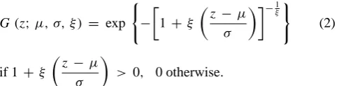
Fig. 1. Illustration of the GEV distribution. Upper panel: example of GEV densitiesf (x;µ,σ,ξ )when varying the locationµparameter

(left plot), the scaleσparameter (middle plot) or the shapeξparameter (right plot). Lower panel: corresponding return level plots.

approximately given by the GEV distribution, with cumula-tive distribution function:

G (z;µ, σ, ξ ) = exp

(

−

1 +ξ

_z−µ

σ

−1_ξ)

(2)

if 1+ ξ

_z−µ

σ

> 0, 0 otherwise.

The GEV distribution has three parameters (Eq. 2): a loca-tion parameterµ, a scale parameterσ >0 and a shape pa-rameterξ. The location specifies where the distribution is centered and the scale its spread. The shape parameterξ de-scribes the tail behavior of the distribution, leading to three types of GEV distributions:

– whenξ >0, a heavy-tailed (or Fr´echet) distribution,

– whenξ=0, a light-tailed (or Gumbel) distribution,

– whenξ <0, a bounded (or Weibull) distribution.

The Gumbel distribution withξ=0 is interpreted in Eq. (2) as the limit whenξ→0, leading to the distribution function

G (z;µ, σ, ξ = 0) = exp

−exp

−

_{z −µ}

σ

.

In case of a bounded distribution (Weibull,ξ <0), the vari-able of interestZnhas a finite upper point, meaning that theo-retically no value above this upper bound can be observed. A light tailed distribution (Gumbel,ξ=0) has an infinite upper point and any value could theoretically be observed. Never-theless, very extreme values (i.e. far from average observa-tions) are very rare. In a heavy-tailed distribution (Fr´echet,

ξ >0), such extremes are still rare but more probable. An

illustration of the influence of the three GEV parameters is depicted in Fig. 1, upper panel, for arbitrary snow-like GEV parameters.

In practice return levels are commonly used for opera-tional purposes. The return levelqpassociated with the re-turn period _p1 (0< p≤1) is the(1−p)-th quantile of the GEV distribution; it is expected to be exceeded on average once every _p1 years. Estimates of return levels are obtained by setting in Eq. (2)G(qp;µ, σ, ξ )=1−pand by inverting it:

qp =

_µ− σ

ξ [1 − {−log(1 −p)}

−ξ_{],forξ 6= 0,}

µ−σ log{−log(1 −p)}, forξ = 0. (3)

The graph of qp against−log(1−p) on a logarithm scale (i.e. the plot ofqpagainst log{−log(1−p)}) is a return level plot. It is particularly convenient for interpreting extreme value models. It gives, for any return periodron the x-axis, the associated return level, i.e. roughly speaking the highest value expected to be exceeded once everyryears (for yearly maxima data). From Eq. (3), ifξ <0 the plot is convex with asymptotic limit asp→0 (infinite return period, i.e. r→ ∞) atµ−σ

ξ; ifξ >0 the plot is concave and has no finite

bound; ifξ=0 it is linear. An illustration is given in Fig. 1, lower panel. It is usually long return periods, corresponding to small values ofp, that are of greatest interest. Cases when

ξ is positive are of particular concern for risk management because very extreme events may occur.

2530 J. Blanchet and M. Lehning: Mapping snow depth return levels

(a) (b)

200 500 1000 1500 2000 2500 3000 3500 4000 50 km

Altitude (m)

200 500 1000 1500 2000 2500 3000 3500 4000 50 km

Altitude (m)

(c) (d)

Altitude (m)

Frequency

0 1000 2000 3000 4000

0

1000

2000

3000

4000

5000

Altitude (m)

Frequency

0 1000 2000 3000 4000

0

2

4

6

8

10

Fig. 2. Upper row: (a) Elevation map of Switzerland and (b) station locations. Lower row: (c) Histogram of

elevations in Switzerland in a1km grid spacing and (d) of the stations. Color indicates elevation in meters

above sea level. Among the100stations,16are excluded from the analysis for validation (red circles in the

right map corresponding to dashed part of the right histogram).

30

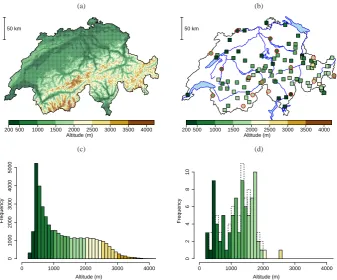
Fig. 2. Upper row: (a) elevation map of Switzerland and (b) station locations. Lower row: (c) histogram of elevations in Switzerland in a

1 km grid spacing and (d) of the stations. Color indicates elevation in meters above sea level. Among the 100 stations, 16 are excluded from the analysis for validation (red circles in the right map corresponding to dashed part of the right histogram).

3 Data

We shall consider annual maximum snow depth from the 100 sites in Switzerland shown in Fig. 2. The stations we consider belong to two manual networks run by SLF (WSL Institute for Snow and Avalanche Research) and MeteoSwiss (Swiss Federal Office for Meteorology and Climatology). Annual maxima are extracted from daily snow depth mea-sured manually on a stake at around 07:30 a.m. during the winter season, i.e. between 1 November and 30 April, for the winters 1965–1966 to 2007–2008. The study area covers all of Switzerland with a higher density in the alpine part; see maps of Fig. 2. The area is characterized by a high den-sity of population, tourism infrastructure and traffic during winter. The elevations of the stations range between 250 m and 2500 m a.s.l. (above sea level), with only two stations above 2000 m. 16 of these 100 stations are excluded from the analysis for validation, and thus 84 are used for inference. These 16 stations have been chosen to cover most of Switzer-land and are located at various elevations between 300 and 2000 m. Some of these chosen stations are purposely cli-matologically unique. For example, the easternmost of the validation stations is the only one in a valley system with a special local climatology; or the westernmost of the vali-dation stations is located at least 500 m higher than all the

surrounding stations in a larger region. The choice of these “unique” stations was made in order to assess performance of the spatial model in the most difficult case. This has to be taken into account when interpreting results for the validation stations in Sects. 5 and 6.

LetZ(s)denote the annual maximum snow depth at sites

of Switzerland, i.e.

Z(s) = max{Y1(s), ..., YL(s)}, (4)

whereYl(s)≥0 denotes the snow depth at sitesthel-th day of the winter (l∈ {1,...L}) andL=181 or 182 denote the number of days in the six winter months from November to April (note that for shortness, indexLinZ(s)is omitted). The processZ= {Z(s), s∈S}whereSdenotes Switzerland can be assumed to be a continuous process, i.e. a smoothly varying process over space. In the context of extreme value theory, this means thatZ(s) can be approximated through a GEV distribution where parameters µ(s), σ (s) andξ(s)

0.2 1.0 5.0 20.0 100.0

0

20

40

60

80

Return period (years)

Return level (cm)

µ=7.42 (1.2)

σ=6.81 (1.17)

ξ=0.52 (0.16)

+ + ++ + + + +

+ ++++ ++++ +++₊+++

+++ + + +

+ ++₊++ ++ + +

+ ++ +++

+++ + + +

+ +

+++ ++

+ + ₊+

+ ++₊ ++ + ++₊+ + +

+ + +

+ +

+ ++

Bellinzona (230m)

0.2 1.0 5.0 20.0 100.0

10

20

30

40

Return period (years)

Return level (cm)

µ=10.02 (1.04)

σ=5.82 (0.81)

ξ=0.14 (0.14)

+ + ++ + +₊ ++

++++ ++++ +++₊+++

+++ + + +

+ ++₊++ ++ + +

+ +++ + +₊+++ + + + +

+++ ++

+ + ₊+

+ ++₊ ++ + ++₊+ + +

+ + +

+ +

+ ++

Delémont (416m)

0.2 1.0 5.0 20.0 100.0

50

100

150

200

250

300

Return period (years)

Return level (cm)

µ=122.2 (7.85)

σ=47 (5.36)

ξ=−0.11 (0.08)

+ + ++ + +₊ ++

++++ ++++ +++₊+++

+++ + + +

+ ++₊++ ++ + +

+ +++ + +₊+++ + + + +

+++ ++

+ + ₊+

+ ++₊ ++ + ++₊+ + +

+ + +

+ +

+ ++

Gadmen (1190m)

0.2 1.0 5.0 20.0 100.0

150

200

250

300

350

Return period (years)

Return level (cm)

µ=237.78 (8.11)

σ=49.06 (5.74)

ξ=−0.36 (0.08)

+ + ++ + +₊ ++

++++ ++++ +++₊+++

+++ + + +

+ ++₊++ ++ + +

+ +++ + +₊+++ + + + +

+++ ++

+ + ₊+

+ ++₊ ++ + ++₊+ + +

+ + +

+ +

+ ++

Weissflujoch (2540m)

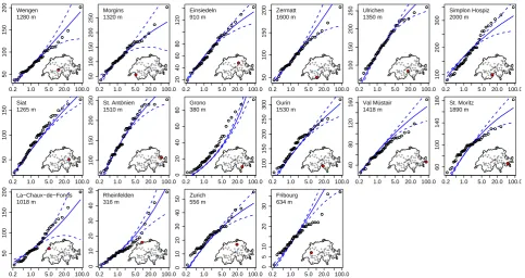
Fig. 3. Snow depth return level plots for four different stations. The blue curve is the GEV-based curve with

standard errors (dashed line). Points are empirical estimates. Locations of the stations are indicated by the red circle in the lower-right Swiss map. Maximum likelihood estimates of the GEV parameters are indicated the upper-left corner (with standard errors).

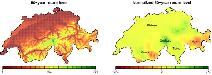
50−year return level

36 226 415

Fig. 4. Pointwise 50-year snow depth return level map (in centimeters).

31

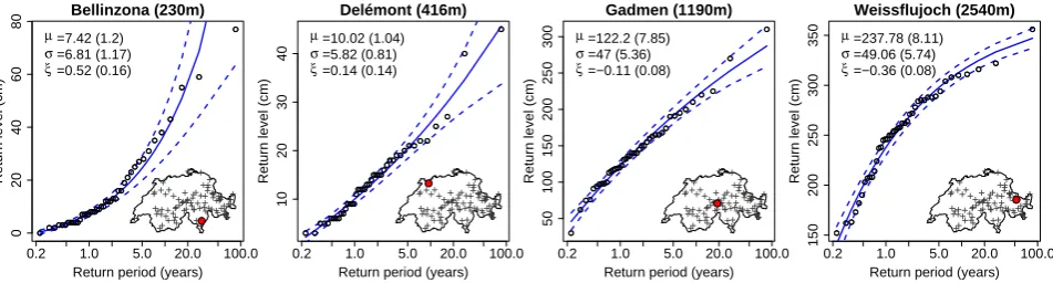
Fig. 3. Snow depth return level plots for four different stations. The blue curve is the GEV-based curve with standard errors (dashed line).

Points are empirical estimates. Locations of the stations are indicated by the red circle in the lower-right Swiss map. Maximum likelihood estimates of the GEV parameters are indicated the upper-left corner (with standard errors).

will allow us to compute return levels for everysin Switzer-land, and therefore to build smooth return level maps.

4 Pointwise estimation of the GEV distributions

Lets1, ..., sN denote theN=84 station locations at hand

(see Fig. 2). We start by studying the pointwise distributions

ofZ(si),i∈ {1, ..., N}. Spatial estimates of these

distribu-tions will be derived in Sects. 5 and 6. As previously stated,

Z(si)is a block maxima random variable given by Eq. (4) where locationsis replaced by locationsi. TheLdaily snow depths Y1(si), ..., YL(si) are dependent random variables due to the strong temporal dependence of snow depth. Never-theless, a separate analysis (not shown) reveals that, for every winter and every locationsi,i∈ {1, ..., N}, the time-series of snow depths exhibit a short-range dependence, which sug-gests that theD(un)condition mentioned in Sect. 2 is satis-fied. Furthermore, the block sizeLon which maximaZ(si) are retrieved is 181 (or 182) corresponding to the six winter months. This size seems to be large enough to assume that the statistical theory of extreme values presented in Sect. 2 applies. Annual maximum snow depth at a given locationsi is then expected to follow a GEV distribution (Eq. 2) with parameters(µi, σi, ξi)to be estimated.

We adopt a maximum likelihood approach. Let

z_i(1), ..., z(K)_i denote the K=43 annual snow depth

max-ima measured at locationsi, i.e. realizations of the random variableZ(si). The log-likelihood for the GEV parameters at stationiis given by:

l (µi, σi, ξi) = −Klogσi −

1 + 1

ξi

K

X

k=1

log (5)

"

1+ξi

z(k)_i −µi

σi

!#

−

K

X

k=1

"

1+ξi

z(k)_i −µi

σi

!#−_ξi1

Maximization of Eq. (5) with respect to the parameter vec-tor(µi, σi, ξi)leads to the maximum likelihood estimate,

denoted by(µˆi,σˆi, ξˆi). There is no analytical solution but the maximization is straightforward using standard numeri-cal optimization algorithms. Rfunctionsfgevin package

evdorfit.gevin packageismevfor example perform this maximum likelihood estimation. Whenξi>−0.5, the maximum likelihood estimate has the usual asymptotic prop-erties (Smith, 1985): µˆi, σˆi and ξˆi are asymptotically un-biased and standard errors are approximately given by the square root of the diagonal of the inverse observed informa-tion matrix (Coles, 2001, chapter 3).

Return levels for stationican then be computed by Eq. (3) where(µ, σ, ξ ) are replaced by the maximum likelihood estimate (µˆi, σˆi, ξˆi). Standard errors and confident in-tervals can also be obtained with the delta method (Coles, 2001, chapter 3). For illustration, return levels plots for four stations at low, middle and high altitude are depicted in Fig. 3, together with empirical estimates of return levels. These plots can also be used for model validation. If the GEV model is suitable for the data, the model-based curve and empirical estimates should be in reasonable agreement. Figure 3 suggests a reasonably good adequacy of the GEV model, even at low altitudes where daily snow depth time-series show a longer time dependence.

An interesting result is that the shape parameters ξi are usually positive at low altitudes, close to 0 at middle altitudes (about 1000 m) and negative at higher altitudes, as illustrated in Fig. 3. The positivity ofξi means that at low altitudes, the distribution of annual maximum snow depth is heavy tailed, i.e. that very large snow depth compared to “usual” snow depth can occur. This heaviness is even more pronounced in the low altitude region of Ticino in southern Switzerland (see Bellinzona compared to Del´emont in Fig. 3) where very intense snowfalls sometimes occur due to the vicinity of the Mediterranean sea and the steep topography. By contrast, at high altitudes the GEV distribution is bounded (see Weissflu-joch in Fig. 3), meaning that no real extremes occur with re-gards to other events. Similar results were found in Blanchet et al. (2009) regarding extreme snowfall in Switzerland.

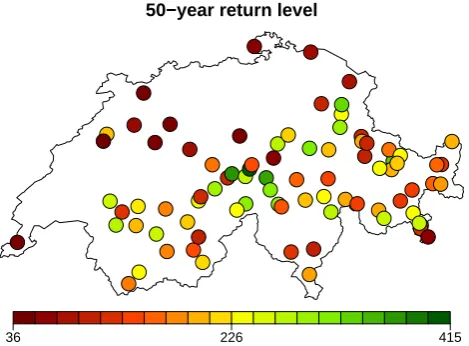
2532 J. Blanchet and M. Lehning: Mapping snow depth return levels Figure 4 depicts the 50-year return levels obtained from

the fitted GEV distributions at theN=84 station locations. Such a map is nevertheless difficult to interpret and can only give information for the few locations where data are avail-able. In practice spatial return levels rather than pointwise estimates would be of much higher value. The rest of this paper will be devoted to this issue.

5 Interpolating the GEV parameters

With the aim of producing return level maps, we would like to have estimates of the smooth surfacesµ(s), σ (s), ξ(s)

for every locationsin Switzerland. The pointwise analysis of Sect. 4 allowed us to have estimates at isolated locations. The most naive way of deriving spatial estimates forµ,σ

andξ is to spatially interpolate the point estimatesµˆi,σˆi,ξˆi,

i∈ {1,...,N}. This is the subject of this section where

differ-ent interpolation techniques are compared. This is also the approach adopted in Kohnov´a et al. (2009) and Beguer´ıa and Vicente-Serrano (2006) both regarding precipitation. Here the functions to be interpolated are then the three GEV pa-rametersµ,σ,ξ. They are assumed to be known at all station locationssi,i∈ {1,...,N}with valuesµˆi,σˆi,ξˆi of Sect. 4. The interpolation problem consists of specifying values at arbitrary locationss∈S. In the followingηwill denote one of the three functionsµ,σandξ to be interpolated andηˆiits known value at locationsi. The goal is then to get smooth estimatesη(s)˜ for all locationss in Switzerland, based on valuesηˆi,i∈ {1, ..., N}.

5.1 Interpolation methods

We give in this section a general overview of the different interpolation techniques that will be used for interpolating the GEV parameters.

5.1.1 Inverse distance weighted

In inverse distance weighting (IDW), interpolated values are a function of the distance to surrounding locations. The in-verse distance weight is used to attenuate the influence of distant points. The interpolated valueηat locationsis given by:

˜

η(s) =

PN

i=1

ˆ ηi

||s−si||

PN

i=1 ||s−1si||

, (6)

where||s−si||is the distance from the interpolating location

si to the interpolated locations. Often the squared distance is used. IDW is an exact interpolation: at station location

si, interpolated valueη(s˜ i)given by Eq. (6) is equal to the known valueηˆi used in the interpolation.

0.2 1.0 5.0 20.0 100.0

0

20

40

60

80

Return period (years)

Return level (cm)

µ=7.42 (1.2)

σ=6.81 (1.17)

ξ=0.52 (0.16)

+ + ++ + +₊ ++

++++ ++++ ++₊₊+++

+++ + + +

+ ++ + + + ++ + +

+ ++ +++++++ + + + +

+++ ++

+ + ₊+

+ ++₊ ++ + ++++ + +

+ + +

+ +

+ ++

Bellinzona (230m)

0.2 1.0 5.0 20.0 100.0

10

20

30

40

Return period (years)

Return level (cm)

µ=10.02 (1.04)

σ=5.82 (0.81)

ξ=0.14 (0.14)

+ + ++ + +₊ ++

++++ ++++ ++₊₊+++

+++ + + +

+ ++ + + + ++ + +

+ +++ + +₊+++ + + + +

+++ ++

+ + ₊+

+ ++₊ ++ + ++++ + +

+ + +

+ +

+ ++

Delémont (416m)

0.2 1.0 5.0 20.0 100.0

50

100

150

200

250

300

Return period (years)

Return level (cm)

µ=122.2 (7.85)

σ=47 (5.36)

ξ=−0.11 (0.08)

+ + ++ + +₊ ++

++++ ++++ ++₊₊+++

+++ + + +

+ ++ + + + ++ + +

+ ++ +++++++ + + + +

+++ ++

+ + ₊+

+ ++₊ ++ + ++++ + +

+ + +

+ +

+ ++

Gadmen (1190m)

0.2 1.0 5.0 20.0 100.0

150

200

250

300

350

Return period (years)

Return level (cm)

µ=237.78 (8.11)

σ=49.06 (5.74)

ξ=−0.36 (0.08)

+ + ++ + +₊ ++

++++ ++++ ++₊₊+++

+++ + + +

+ ++ + + + ++ + +

+ ++ +++++++ + + + +

+++ ++

+ + ₊+

+ ++₊ ++ + ++++ + +

+ + +

+ +

+ ++

Weissflujoch (2540m)

Fig. 3. Snow depth return level plots for four different stations. The blue curve is the GEV-based curve with

standard errors (dashed line). Points are empirical estimates. Locations of the stations are indicated by the red circle in the lower-right Swiss map. Maximum likelihood estimates of the GEV parameters are indicated the upper-left corner (with standard errors).

50−year return level

36 226 415

Fig. 4. Pointwise 50-year snow depth return level map (in centimeters).

31

Fig. 4. Pointwise 50-year snow depth return level map (in

centime-ters).

5.1.2 Linear regression models

Letx1,s, ..., xp,sdenotepexploratory variables known for

the whole of Switzerland (i.e. for eachs∈S). For example thep=3 exploratory variables of longitude, latitude and el-evation could be used, or polynomials of these variables. To predictηat sitesgivenx1,s, ..., xp,sone might consider the following model:

η(s) = β0+β1x1,s + ... +βpxp,s +s, (7)

whereβ0, β1, ..., βp are the regression parameters to be estimated ands is an error term. Errorss are supposed to follow the ordinary least squares assumptions, in particular to be i.i.d. The model is estimated by minimizing with respect to theβs the least squares error at locationssi,i∈ {1,...,N}, where valuesηˆi ofη(si)are known. This gives least square estimatesβ˜0, β˜1, ...,β˜p. The predicted value at unknown locationsis then given by

˜

η(s) = ˜β0 + ˜β1x1,s + ... + ˜βpxp,s (8)

This is not an exact interpolation: at station locationsi, pre-dicted valueη(s˜ i)given by Eq. (8) and known valueηˆi are usually not equal (the error is given bysi of Eq. 7).

5.1.3 Spline-based regression model

Consider the nonparametric regression model defined as

η(s) = F x1,s, ..., xp,s

+s (9)

may modelF as a smooth non-linear function of the covari-ates x’s. A particularly convenient model results when F

is taken as a penalized spline (P-spline henceforth) with ra-dial basis function of orderp, pbeing odd (Marx and Eil-ers, 1998). Estimation of Eq. (9) based on known valuesηˆi is then performed by minimizing the sum of squared errors subject to some constraints to avoid overfitting. Technical details can be found in Appendix A.

A drawback of model Eq. (9) is that estimation may in-volve a very large number of free parameters, even for a low numberpof covariatesx1,s, ..., xp,s. In order to reduce the number of parameters to be estimated while still using thep

covariatesx1,s, ..., xp,s, one may combine the approaches Eqs. (7) and (9) by considering a partially linear model of the form

η(s)=β0+β1x1,s+...+βqxq,s+F xq+1,s, ..., xp,s+s

(10) whereF is a P-spline. Equation (10) belongs then to the family of generalized additive models (GAM) of Hastie and Tibshirani (1990). Estimation and prediction of such a model can be performed similarly to the spline regression model Eq. (9) by using a straightforward modification of matrix X of Appendix A. If_β˜_{s denote the estimate of βs andF}˜ _the

estimated P-spline in Eq. (10) then predicted value ofηat locationsis given by

˜

η(s)= ˜β0+ ˜β1x1,s+...+ ˜βqxq,s+ ˜F xq+1,s, ..., xp,s

.

(11) This is usually not an exact interpolation (error at locationsi is given bysi of Eq. 10).

5.1.4 Kriging

Kriging is a stochastic interpolation method that computes the best linear unbiased estimatorη(s)˜ of η(s)based on a Gaussian model of the spatial dependence. Different kinds of kriging methods exist depending on the assumptions about the mean structure

whereFis a function andǫsis an error term. Errorsǫsare supposed to follow the classical regression

assumptions, in particular to be i.i.d. IfF is linear with respect to each variablex, then (9) is the

linear regression model of (7). For a more complex behavior than a linear dependence, one may

modelF as a smooth non-linear function of the covariatesx’s. A particularly convenient model

results whenF is taken as a penalized spline (P-spline henceforth) with radial basis function of 215

orderp,pbeing odd (Marx and Eilers, 1998). Estimation of (9) based on known valuesηˆiis then

performed by minimizing the sum of squared errors subject to some constraints to avoid overfitting.

Technical details can be found in Appendix A.

A drawback of model (9) is that estimation may involve a very large number of free parameters,

even for a low numberpof covariatesx1,s,...,xp,s. In order to reduce the number of parameters

to be estimated while still using thepcovariatesx1,s,...,xp,s, one may combine the approaches (7)

and (9) by considering a partially linear model of the form

η(s) =β0+β1x1,s+...+βqxq,s+F(xq+1,s,...,xp,s) +ǫs (10)

whereF is a P-spline. Equation (10) belongs then to the family of generalized additive models

(GAM) of Hastie and Tibshirani (1990). Estimation and prediction of such a model can be performed

similarly to the spline regression model (9) by using a straightforward modification of matrixXof Appendix A. Ifβ˜s denote the estimate ofβs andF˜the estimated P-spline in (10) then predicted value ofηat locationsis given by

˜

η(s) = ˜β0+ ˜β1x1,s+...+ ˜βqxq,s+ ˜F(xq+1,s,...,xp,s). (11)

This is usually not an exact interpolation (error at locationsiis given byǫsiof equation 10).

5.1.4 Kriging

220

Kriging is a stochastic interpolation method that computes the best linear unbiased estimatorη˜(s)of

η(s)based on a Gaussian model of the spatial dependence. Different kinds of kriging methods exist depending on the assumptions about the mean structureE[η(s)]of the model. The most general case, universal kriging, assumes that the mean is unknown but depends linearly onpcovariates

x1,s,...,xp,s

E[η(s)] =β(s)≡β0+β1x1,s+...+βpxp,s, (12)

where coefficientsβs have to be estimated. In other words,ηat locationsis modeled as

η(s) =β0+β1x1,s+...+βpxp,s+F(s) (13)

where{F(s),s∈ S}is a zero-mean Gaussian process. Model (13) belongs to the family of gener-alized linear geostatistical models as described by Diggle and Ribeiro (2007). Equations (10) and

(13) are similar but differ in that in the formerFis deterministic (a P-spline) whereas in the latter

9

[η(s)]of the model. The most general case, universal kriging, assumes that the mean is unknown but depends linearly onpcovariatesx1,s, ..., xp,s

whereFis a function andǫsis an error term. Errorsǫsare supposed to follow the classical regression

assumptions, in particular to be i.i.d. IfF is linear with respect to each variablex, then (9) is the

linear regression model of (7). For a more complex behavior than a linear dependence, one may

modelF as a smooth non-linear function of the covariatesx’s. A particularly convenient model

results whenF is taken as a penalized spline (P-spline henceforth) with radial basis function of 215

orderp,pbeing odd (Marx and Eilers, 1998). Estimation of (9) based on known valuesηˆiis then

performed by minimizing the sum of squared errors subject to some constraints to avoid overfitting.

Technical details can be found in Appendix A.

A drawback of model (9) is that estimation may involve a very large number of free parameters,

even for a low numberpof covariatesx1,s,...,xp,s. In order to reduce the number of parameters

to be estimated while still using thepcovariatesx1,s,...,xp,s, one may combine the approaches (7)

and (9) by considering a partially linear model of the form

η(s) =β0+β1x1,s+...+βqxq,s+F(xq+1,s,...,xp,s) +ǫs (10)

whereF is a P-spline. Equation (10) belongs then to the family of generalized additive models

(GAM) of Hastie and Tibshirani (1990). Estimation and prediction of such a model can be performed

similarly to the spline regression model (9) by using a straightforward modification of matrixXof Appendix A. Ifβ˜s denote the estimate ofβs andF˜the estimated P-spline in (10) then predicted value ofηat locationsis given by

˜

η(s) = ˜β0+ ˜β1x1,s+...+ ˜βqxq,s+ ˜F(xq+1,s,...,xp,s). (11)

This is usually not an exact interpolation (error at locationsiis given byǫsiof equation 10).

5.1.4 Kriging

220

Kriging is a stochastic interpolation method that computes the best linear unbiased estimatorη˜(s)of

η(s)based on a Gaussian model of the spatial dependence. Different kinds of kriging methods exist depending on the assumptions about the mean structureE[η(s)]of the model. The most general case, universal kriging, assumes that the mean is unknown but depends linearly onpcovariates

x1,s,...,xp,s

E[η(s)] =β(s)≡β0+β1x1,s+...+βpxp,s, (12)

where coefficientsβs have to be estimated. In other words,ηat locationsis modeled as

η(s) =β0+β1x1,s+...+βpxp,s+F(s) (13)

where{F(s),s∈ S}is a zero-mean Gaussian process. Model (13) belongs to the family of gener-alized linear geostatistical models as described by Diggle and Ribeiro (2007). Equations (10) and

(13) are similar but differ in that in the formerF is deterministic (a P-spline) whereas in the latter

9

[η(s)] = β(s) ≡ β0 +β1x1,s + ... +βpxp,s, (12) where coefficientsβs have to be estimated. In other words,η

at locationsis modeled as

η(s) = β0 +β1x1,s + ... +βpxp,s +F (s) (13)

where{F (s), s∈S}is a zero-mean Gaussian process. Model Eq. (13) belongs to the family of generalized linear geosta-tistical models as described by Diggle and Ribeiro (2007). Equations (10) and (13) are similar but differ in that in the formerF is deterministic (a P-spline) whereas in the latter

F is stochastic (a Gaussian process). A formal connection between spline and kriging exists, see for example Cressie (1993), p. 180 and references therein.

Estimation of Eq. (13) involves estimating theβs parame-ters and the variogram describing the dependence structure in the Gaussian processF, which can be realized by maximum likelihood (see Diggle and Ribeiro, 2007, chapter 5). The minimum mean square error predictorη˜ofηat locationsis then given by an equation of the form (Diggle and Ribeiro, 2007, chapter 6)

˜

η(s) = ˜β(s) +

N

X

i=1

wi(s){ ˆηi − ˜β(s)} (14)

where_β(s)˜ _{is the estimated mean at location s and w}

i(s) are called prediction weights. This shows that the predicted valueη(s)˜ is basically a weighted mean of the known val-uesηˆi. However, unlike IDW of Sect. 5.1.1, weightswi(s),

i∈ {1,...,N}, depend on the target locations. These weights

can be positive, zero or negative depending on the correlation between locationssandsi. When no nugget effect is consid-ered (i.e. when the variogram is supposed to be continuous at the origin), kriging is an exact interpolation method.

5.2 Choice of covariates

The interpolation methods presented in the previous sec-tion are applied for interpolating the three GEV parameters, i.e. withη being either the locationµparameter, the scale

σ parameter, or the shapeξ parameter. The first question to answer regards the choice of the covariatesx.,s to be used. As the final goal of this work is the mapping of return levels, maps of these covariates would be needed, or at least gridded values in Switzerland.

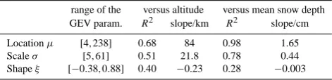
It is natural to consider the three geographical coordinates (longitude, latitude, altitude) as covariates in the interpola-tion methods. For snow events, altitude plays the most im-portant role. As shown in Table 1, there is a strong linear dependence of the GEV parameters with altitude. The mag-nitude (modeled byµ) and spread (modeled byσ) of extreme snow depth strongly increase with elevation. On the contrary, as discussed in Sect. 4,ξ basically decreases with elevation, with positive values (heavy tailed distributions) at low alti-tudes and negative values (bounded distributions) at high al-titudes. Similar results were found in Blanchet et al. (2009) regarding extreme snowfall in the Swiss Alps.

Additional covariates may help the prediction of extreme snow depth. Table 1 reveals that for the location and scale parameters, the mean snow depth is even more informa-tive than elevation (higher R2). The importance of mean snow depth shows that snow distribution in Switzerland can-not be completely described by the three geographical co-ordinates. Mean snow depth may contain additional infor-mation on local maxima and minima in snow distribution such as caused by individual mountain ranges. The positive

2534 J. Blanchet and M. Lehning: Mapping snow depth return levels

Table 1. Summary of linear dependence of the GEV parameters

of Sect. 4 with altitude (columns 3 and 4) and with the mean snow depth (columns 5 and 6). In all cases, covariates are very

signifi-cant (p-values lower than 10−6). Altitude ranges between 230 and

2540 m, mean snow depth between 0.5 and 146 cm. The range of

theN=84 estimated GEV parameters is indicated in the first

col-umn.

range of the versus altitude versus mean snow depth GEV param. R2 slope/km R2 slope/cm

Locationµ [4,238] 0.68 84 0.98 1.65

Scaleσ [5,61] 0.51 21.8 0.78 0.44

Shapeξ [−0.38,0.88] 0.40 −0.23 0.28 −0.003

correlation between mean snowfall and the location param-eter µ of extreme snowfall has already been discussed by Blanchet et al. (2009) and it is therefore reasonable to have a positive correlation between mean and extreme snow depth as well. It is also reasonable to have a generally wider dis-tribution of snow depth values if snow depth is large, i.e. a positive correlation between mean snow depth and the scale parameter,σ. Note, however, that for both snowfall and snow depth the shape parameter,ξ, is negatively correlated to the mean as discussed in Blanchet et al. (2009). This is partly a result of having many zero-events (rain instead of snow and zero snow depths) and a few much larger events for stations with a low mean.

To use it as a possible covariate in the spatial interpolation, a map of the mean snow depth is needed, which is not avail-able. However, the mean snow depth is a very smooth pro-cess, even much smoother than a one-day event process such as maximum annual values or daily values. Its spatial inter-polation is therefore easier than mapping daily snow depth as in Erxleben et al. (2002), Molotch et al. (2005) or Foppa et al. (2007) for example. A universal kriging interpolation (see section 5.1.4) with a linear trend on altitude gives very accurate interpolated mean values, with a root mean squared error (RMSE) of less than 5 cm (not shown). Using a digital elevation model (DEM henceforth) of Switzerland, gridded maps of mean snow depth can then be obtained and used as covariate for the location and scale GEV parameters.

Other meteorological variables, such as wind speed, wind direction and temperature, are also measured at the station lo-cations. Nevertheless, a separate analysis did not reveal any significant influence of these variables on the GEV parame-ters. This may be partly due to the poor quality of these data and to the fact that many values are missing. Topographical variables such as slope, aspect, net solar radiation or vegeta-tion used in Erxleben et al. (2002), Molotch et al. (2005), or Gr¨unewald et al. (2010) could also be used as supplementary information, but are not considered in this work. Since lo-cal topographilo-cal variables are already of limited use in fine-scale snow depth analysis (Gr¨unewald et al., 2010), we do

not expect them to help explain our snow depth data, which are collected on flat fields. We will return to this point in the discussion (Sect. 7). Here the considered covariates for in-terpolating the GEV parameters are then the four covariates longitude, latitude, altitude and mean snow depth.

5.3 Considered models

We detail below the models used for interpolating the GEV parameters. As in Sect. 5.1, we denote ηany of the three functionsµ,σ orξ to be interpolated. For sake of concise-ness, we only detail in this section models when the four co-variates longitude, latitude, altitude and mean snow depth are considered. Embedded models (in particular models when the mean snow depth is not accounted for) are particular cases which are straightforward to derive.

5.3.1 Inverse distance weighting

In order to account for the strong dependence of the GEV parameters with altitude and mean snow depth, one might rather use IDW with gradient correction as proposed in e.g. Nalder and Wein (1998):

˜

η(s) =

PN

i=1

ˆ

ηi+βa as −a_si+βm ms−m_si

||ls−l_si||

PN

i=1 ||ls−1l_si||

, (15)

whereasis the altitude of locations,msits mean snow depth,

ls is the two-dimensional coordinate of this site (longitude, latitude),βa andβm are parameters. Compared to Eq. (6), Eq. (15) has the advantage of giving more weight to altitude and mean snow depth. This corrected IDW method is still an exact interpolation. Parametersβaandβmcan be estimated by cross-validation by choosing values minimizing the score

CV (βa, βm)=

N

X

i=1

(ηˆi− ˜η−i(si))2,

whereη˜−i(si)is the interpolated value at sitesi when this station is omitted in Eq. (15).

5.3.2 Linear regression models

Models of the form Eq. (7) are used where the covariates are polynomials of longitude, latitude, altitude and mean snow depth with a maximum degree of 3. We consider all possible combinations of these covariates with a maximum number of covariates (pin Eq. 7) equal to 6. We select the “best” linear regression model with the help of AIC, a penalized likelihood criteria (Akaike, 1974). Results of Sect. 5.5 will correspond to this model.

5.3.3 Spline regression models

We use models of the form

whereF is a P-spline of order 3. Spline-regression models require to choose fix knots (see Appendix A). Choosing the best number of knots, and the best locations for them, is a difficult task. Here we fixed the number of knots to 15 which seems to be a good compromise between flexibility (large number of knots) and simplicity (low number of knots) of the model. These 15 knots are considered among theN=84 station locations only. The best position for these 15 knots, from 10 000 of the total of 84₁₅possibilities, is made by gen-eralized cross-validation. More precisely, 10 000 estimations with different choices of positions for the 15 knots are per-formed. Among the 10 000 estimated models, the one with the lowest GCV value (see Appendix A) is selected as the “best” model and results of Sect. 5.5 will correspond to this model.

5.3.4 Kriging

Model Eq. (16) is used withF being a Gaussian process with mean zero. No nugget effect is considered here, i.e. the var-iogram modeling the dependence structure is supposed to be continuous at the origin. Computation of this variogram in-volves the choice of a covariance function forF. Nine of the most commonly used covariance functions are used, namely the spherical, circular, cubic, Gneiting, exponential, Mat´ern, Gaussian, powered-exponential and Cauchy covariance func-tions (Schabenberger and Gotway, 2005). These covariance functions have one or two degrees of freedom and the four first ones have an upper-bound. Maximum likelihood es-timation is performed with library geoRof R. The “best” model (i.e. the best covariance function) is then selected with the help of the AIC criteria (Akaike, 1974). Note that as no nugget effects are used here, kriging is an exact interpolation method.

5.4 Prediction comparison

To assess quality of the predictions, measures of accuracy will be used. The most stringent comparison is obviously to compute such measures for the validation stations. Note that validation stations were mainly selected for their climatolog-ical properties and not in order to achieve a high score in the validation (see Sect. 3). Therefore, the validation tests the reliability and stability of the predictions over all of Switzer-land, or at least below 2500 m. However, it may also be of interest to assess the quality of the interpolated distributions for the fitted stations, in particular for the linear and spline regression models which are non-exact methods. Large dif-ferences between measures for theN=84 fitting stations and theM=16 validation stations indicate models that are ques-tionable.

Here four measures of accuracy are used: the root mean-squared error (RMSE), the mean absolute error (MAE), the maximum prediction error (MPE) and the bias. These measures could be computed for assessing quality of the

interpolatedµ(s˜ i),σ (s˜ i)andξ (s˜ i)compared respectively to the individual valuesµˆi, σˆi andξˆi of Sect. 4. This would however result in a comparison between two estimators, and not between an estimator and an observation. Furthermore, strictly speaking, it would not answer the question as to how well the data distribution is captured: the three best mod-els forµ, σ andξ separately might not be the best triplet

of (µ, σ, ξ )since the GEV parameters are not orthogonal

parameters. A better comparison is to assess goodness-of-fit of the quantiles of the interpolated GEV distribution com-pared to the observed ones. Letz(_i1), ..., z(K)_i be theK=43 quantiles (i.e. sorted values) observed at a given station i. The probability associated to the k-th valuez(k)_i is usually

pk=k−_K1/2 (functionppointsinR).z(k)_i can therefore be compared with the(1−pk)quantile of the interpolated GEV distribution at stationi, denotedq˜pk,i. It is given by Eq. (3),

where µ, σ and ξ are replaced by their interpolated val-ues µ(s˜ i), σ (s˜ i)and ξ (s˜ i) and p is replaced by pk. The goodness-of-fit scores for quantile comparison are then given by

RMSE = v u u t

1

N K

N

X

i=1 K

X

k=1

z(k)_i − ˜qpk,i

2

,

MAE = 1

N K

N

X

i=1 K

X

k=1

|z(k)_i − ˜qpk,i|,

MPE = maxi∈{1,...,N}maxk∈{1,...,K}|z_i(k) − ˜qpk,i|,

Bias = 1

N K

N

X

i=1 K

X

k=1

z(k)_i − ˜qpk,i

.

All these criteria involve quantities of the form (z(k)_i − ˜

qpk,i)which is the error of predicting the(1−pk)quantile

of station i when using the interpolated GEV distribution. Quantile comparison should be made for both theN=84 fit-ting stations and theM=16 validation stations (replacingN

byM is the previous scores). Note that, in the context of extremes, an alternative quantile validation score is used in Friederichs and Hense (2007) and in Maraun et al. (2010), still based on differences of the form(z(k)_i − ˜qpk,i)but where

cases of overestimation (i.e. when z_i(k)− ˜qpk,i<0) and of

underestimation (i.e. whenz(k)_i − ˜qpk,i>0) of the observed

quantilesz(k)_i are differently penalized. There is no reason to use this additional functionality in our case.

5.5 Results

The different interpolation methods presented in Sect. 5.3 are used for interpolating the three GEV parameters. Tables 2 and 3 summarize the scores of Sect. 5.4. In Table 2 only a DEM is used as covariates for the three GEV parameters. In Table 3, the mean snow depth is used as additional covariate

2536 J. Blanchet and M. Lehning: Mapping snow depth return levels

Table 2. Scores of quantile comparison when (a) fitting a GEV to each station separately as in Sect. 4; (b)–(e) interpolating the GEV

parameters with a DEM as covariate.

Fitting stations Validation stations

RMSE MAE MPE Bias RMSE MAE MPE Bias

(a) Pointwise GEV 6.7 3.6 227.9 0.1 5.4 3.3 53.0 0.2

(b) IDW 6.7 3.6 227.9 0.1 17.7 14.8 62.5 −2.2

(c) Linear regression 34.7 26.7 234.6 0.4 33 27.9 107.3 −4.8

(d) Spline regression 19 14.4 131.2 0.2 27.5 21.7 102.7 −6.4

(e) Kriging 6.7 3.6 227.9 0.1 16.2 12.7 71.6 −1.3

Table 3. Scores of quantile comparison when using a DEM and the mean snow depth as covariates. For the validation stations, either the

kriged mean snow depths or the observed mean snow depths (scores in brackets) are used. Methods (a) to (d) are interpolation methods of Sect. 5. Method (e) refers to Sect. 6.

Fitting stations Validation stations

RMSE MAE MPE Bias RMSE MAE MPE Bias

(a) IDW 6.7 3.6 227.9 0.1 14.0 (12.8) 10.3 (9.3) 69.9 (68.8) −1.1 (−0.5)

(b) Linear regression 10.7 6.6 181.7 0.3 13.5 (12.1) 10.1 (8.9) 73.5 (72.6) −1.2 (−0.7)

(c) Spline regression 9.5 6.0 123.1 0.2 12.8 (11.6) 9.3 (8.1) 87.5 (86.6) −1.0 (−0.5)

(d) Kriging 6.7 3.6 227.9 0.1 12.9 (11.7) 9.4 (8.2) 61.9 (60.9) −0.7 (−0.4)

(e) Smooth GEV 8.6 5.7 118.9 0.3 9.2 (8.3) 6.5 (5.4) 50.9 (48.6) 1.0 (0.6)

for the location and scale parameters, using either the kriged mean values (see Sect. 5.2) or the observed ones. For com-parison, we also indicate in Table 2 the scores correspond-ing to fittcorrespond-ing a GEV distribution to each station separately, including the validation stations, without any spatial model (see Sect. 4). For the validation stations, these scores thus do not correspond to predictions but to fittings, unlike all the other scores (lines b to e). They can thus only be interpreted as lower bounds of the error that would result from a predic-tion.

Table 2 suggests that, when using only longitude, latitude and elevation as covariates, kriging performs better as almost all scores are lower. IDW is the second best model. For both methods, results for the validation stations are relatively poor compared to those for the fitting stations, in particular for RMSE and MAE. This suggests that the prediction quickly deteriorates away from the fitting stations. Note that krig-ing and IDW are exact interpolation methods. This implies for example that the interpolated locationµ(s˜ i)for the fitting stationiis equal to the individual valueµˆi used in the inter-polation. The same applies for the scaleσ (s)and shapeξ(s). Interpolated and individual GEV distributions of the fitting stations are then identical (see lines a, b and e of Table 2). These scores are all low, with the exception of a very large MPE value (227.9) due to one single observation at the sta-tion Lugano in southern Ticino. Parameterξi is likely to be overestimated which produces a strong overestimation of the largest observation.

Table 3 (lines a to d) compared to Table 2 confirms that using the mean snow depth as covariate for the location and scale parameters is helpful. There is a clear improvement in the spline and linear regression models for both the fitted and validation stations. For kriging and IDW, results for the validation stations are only slightly better and results for the fitted stations are exactly the same since they are exact inter-polation techniques. All interinter-polation methods now have a similar performance but kriging still performs slightly better. Scores for the validation stations when using the observed mean snow depth as a covariate are better than when using the kriged mean snow depth but differences are low. This confirms again that the kriged mean snow depth is a very ac-curate estimation of the observed mean, as already discussed in Sect. 5.2. Note that even when using the observed mean snow depth, error measures from the smooth model are quite high compared to those when a GEV is fitted to each station separately (first line of Table 2). The errors cannot strictly be compared since the individual GEV fitting uses all available information at the validation stations for parameter estima-tion, while this information is not used in the parameter es-timation of the smooth GEV. However, the difference in the errors shows that further improvements in the spatial aspect of the smooth GEV model may be possible.

Kriging Smooth GEV

50 100 150 200

50

100

150

200

Observed quantiles (cm)

Estimated quantiles (cm) ++ ++ + +₊ ++

++++ +₊

++ ++++ +

+ + +++

+ + +

+ ++ + + + ++ + +

+ +++ + +₊+++ + + + +

+₊+ ++

+ + ₊+

+ ++

+ ++ + ++₊+ + +

+ + +

+ +

+ ++

1018 m

La−Chaux−de−Fonds

0 10 20 30 40 50

0

10

20

30

40

50

Observed quantiles (cm)

Estimated quantiles (cm) ++ ++ + +₊ ++

++++ +₊

++ ++++ +

+ + +++ + + +

+ ++ + + + ++ + +

+ ++ +++++++ + + + +

+₊+ ++

+ + ₊+

+ ++

+ ++ + ++₊+ + +

+ + +

+ +

+ ++

316 m Rheinfelden

0 10 20 30 40 50

0

10

20

30

40

50

Observed quantiles (cm)

Estimated quantiles (cm) ++ ++ + +₊ ++

++++ +₊

++ ++++ +

+ + +++ + + +

+ ++ + + + ++ + +

+ ++ +++++++ + + + +

+₊+ ++

+ + ₊+

+ ++

+ ++ + ++₊+ + +

+ + +

+ +

+ ++

556 m Zurich

0 5 10 15 20 25 30 35

0

5

10

15

20

25

30

35

Observed quantiles (cm)

Estimated quantiles (cm) ++ ++ + +₊ ++

++++ +₊ ++ ++++ +

+ + +++ + + +

+ ++ + + + ++ + +

+ ++ +++++++ + + + +

+₊+ ++

+ + ₊+

+ ++

+ ++ + ++₊+ + +

+ + +

+ +

+ ++

634 m Fribourg

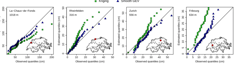
Fig. 5. QQ-plots of all four validation stations located in the Plateau, with kriging interpolation (green squares)

and smooth GEV fitting (blue triangles). With both methods, longitude, latitude and elevation are used as covariates for the GEV parameters. The kriged mean snow depth is an additional covariate for the location and scale. Kriging interpolation is related to section 5. Smooth GEV fitting is related to section 6.

0 20 40 60 80 100 120

35000

35500

36000

Model number

TIC

Model comparison: TIC values

Covariates for σ:

a DEM

a DEM and the mean a DEM and µ

Covariates for µ: a DEM

Covariates for µ: a DEM and the mean

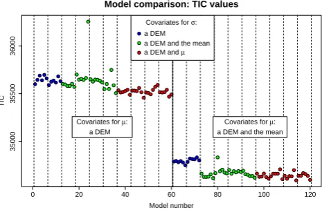
Fig. 6. Model comparison using TIC for two out of the six consideredµmodels. Models1to60use a DEM as covariates for µ; models 61to120use a DEM and the mean snow depth as covariate forµ. Each block delimited by two dotted lines corresponds to a given model forµandσ, when all the six different models forξ

are used.

32

Fig. 5. QQ-plots of all four validation stations located in the Plateau, with kriging interpolation (green squares) and smooth GEV fitting (blue

triangles). With both methods, longitude, latitude and elevation are used as covariates for the GEV parameters. The kriged mean snow depth is an additional covariate for the location and scale. Kriging interpolation is related to Sect. 5. Smooth GEV fitting is related to Sect. 6.

z_i(k),k∈ {1, ...,43}, against the modeled quantilesq˜pk,i: this

is a QQ-plot. Figure 5 (green squares) depicts QQ-plots of all four validation stations located on the Swiss Plateau with kriging interpolation of Table 3. With a perfect fit, all points would lie on the diagonal line. In Fig. 5 the kriged mean snow depth is used as a covariate but results with the ob-served mean are almost similar. The figure reveals that the interpolated GEV distributions in the low elevation Plateau are quite poor. A comparison with QQ-plots of the valida-tion stavalida-tions located in the Alps (not shown) reveals a better fit in the Alps. One reason is that the station network in the Plateau is much less dense than in the Alpine region (see Fig. 2). The interpolation process will then produce a better fit in the Alps than on the Plateau, which has fewer stations. In addition, the statistically more extreme snow depth values on the Plateau (due to positive shape parameters, see Sect. 4) are by their very nature more difficult to model. However, the main drawback of the methodology is that the interpolation is done independently of the data. Of course, individual esti-mationsµˆi,σˆiandξˆiin Sect. 4 were done based on observed data. However, once the GEV parameters are estimated, they are considered as true values in the interpolation process, as if they were really observed. A bad individual estimate will therefore induce a bad interpolated value and may lead to models that are very unlikely for the data. This is no longer the case when a smooth GEV model is directly fitted to the data, as described in the next section.

6 Fitting a smooth GEV model

6.1 Smooth GEV modeling

There are crucial differences between the interpolation meth-ods of Sect. 5. Unlike kriging and IDW, linear and spline regressions are generic models: once the model parameters have been estimated, prediction does not involve the indi-vidual valuesηˆi anymore, which are only used for inference

(see Eqs. 8 and 11 compared to Eqs. 6 and 14). For these two cases, another approach is to directly estimate the regression parameters from the data, without involving the individual valuesηˆi. This method will be termed “smooth GEV mod-eling” because the GEV parameters are directly modeled as smooth functions in space. The main difference with the ap-proach of Sect. 5 is that in interpolation methods, the spatial information is derived by interpolating individual GEV es-timates whereas in the smooth GEV modeling it can be di-rectly estimated from the data. More precisely, letηdenote the surface model for either the locationµ, scaleσ or scale

ξ parameter. We model the surfaceηat locations with the linear model

η(s) = β0+β1x1,s + ... +βpxp,s (17)

as in linear regression prediction (Eq. 8), or with the more general additive model

η(s)=β0+β1x1,s+...+βqxq,s+F xq+1,s, ..., xp,s

(18) where F is a P-spline as in spline regression prediction (Eq. 11). Note that compared to the regression models Eqs. (7) and (10), models Eqs. (17) and (18) are determin-istic as they do not comprise the stochastic part contained in the (Gaussian) residualss.

Smooth spline-based models similar to Eq. (18) have also been used for example in Hall and Tajvidi (2000), Ramesh and Davison (2002) and Padoan and Wand (2008) but for modeling smooth temporal trends of the GEV parameters at individual locations (i.e. with time as a covariate), rather than smooth spatial surfaces as in this article. In the spatial frame-work, recently quite simple linear regression models as in Eq. (17) have been used in Padoan et al. (2010) regarding US precipitation, using only latitude and elevation as covariates. The GEV modeling involves there in total only 7 parame-ters with a constant modelξ(s)=ξ0for the shape. However,

2538 J. Blanchet and M. Lehning: Mapping snow depth return levels only 46 gauging stations were used over an area equivalent

to 10 times Switzerland, with much flatter topography (max-imum elevation around 1500 m). Due to the denser network used in this analysis, the rougher topography and the larger variability of snow depth in Switzerland, the surfaces re-sponses given by Eqs. (17) and (18) to be used on our data are likely to be more complicated, i.e. to involve more covariates

x.,s.

As in Sect. 5, we will consider as possible covariates the three geographical coordinates (longitude, latitude, eleva-tion) and the mean snow depth, with the GEV parameters

µ,σ andξ being modeled by either Eqs. (17) or (18). Each combination of these three models then leads to a smooth GEV modeling of extreme snow depth in Switzerland. How-ever, considering all possible combinations of models forµ,

σ andξ and all possible covariate choices would clearly be too computationally intensive: ifKµmodels are considered forµ,Kσ models forσ andKξ forξ, then in total, by com-bination of all possible models for each of the three parame-ters, this means thatKµ×Kσ×Kξsmooth GEV models have to be fitted. This gives many thousands of models in our case. In order to limit the number of considered GEV mod-els, we restrict our analysis to the best combinations of co-variates found in the previous section using the linear Eq. (7) and spline Eq. (10) regression models. The linear regression models fitted in Sect. 5 used as possible covariate polynomi-als of longitude, latitude, altitude and mean snow depth with a maximum degree of 3 (see Sect. 5.3.2). Spline linear re-gression models used P-spline of order 3 with 15 knots and an additional possible linear dependence in elevation and in the mean (see Sect. 5.3.3). Among all those linear and spline regression models, we only select here as possible models for

µ,σ andξ in the smooth GEV model:

– for the locationµ: the best two regression models with

a DEM as covariate and the best four regression models with a DEM and the mean snow depth as covariates;

– for the scaleσ: the best two regression models with a

DEM as covariate and the best four regression models with a DEM and the mean snow depth as covariates. As

σ (which models the spread of the GEV distribution) andµ(which models the center) are usually very cor-related, we also allow the location to be a covariate for

σby considering the best four regression models with a DEM and the location as covariates;

– for the shapeξ: the best six regression models with a

DEM as covariates.

Note that here only the equations of the best models forµ,

σ andξ are used, and not the values of theβs which will in fact be directly estimated from the data (see Sect. 6.2). This gives a total number of 6×10×6=360 smooth GEV models. These models have between 10 and 57 degrees of freedom. The only model with 57 degrees of freedom is

whenµ,σ andξ are all modeled as in Eq. (18) with a linear dependence with the mean (forµandσ) or with elevation (forξ) and a smooth dependence in space (modeled in Eq.18 through the P-splineF of order 3 with 15 knots).

6.2 Model estimation and selection

Unlike in Sect. 5, we wish to estimate the smooth GEV mod-els directly from the data, which are considered jointly, with-out any individual fitting. We adopt a likelihood approach. This requires to consider the joint distribution of annual max-imum snow depth at theN fitting locations. For the sake of simplicity, we will assume here that theN-variate density can be approximated by the product of marginal densities. This is equivalent to considering that theN annual maxima are approximately independent. This approximation is actu-ally very unlikely to be fulfilled in reality due to the spatial dependence of annual maxima. However, it is applicable and gives satisfying results if the marginal distributions only are of interest, which is the case in this study. We will return to this approximation and its limits in the concluding discus-sion (Sect. 7). The log-likelihood of theN stations is then approximated by

la(µ, σ, ξ ) =

N

X

i=1

l{µ (si), σ (si), ξ (si)} (19)

where µ, σ and ξ are smooth surfaces and

l{µ(si), σ (si), ξ(si)} is the GEV log-likelihood of

Eq. (5) when parameters (µi, σi, ξi) are replaced by

(µ(si), σ (si), ξ(si)). Approximation Eq. (19) is a special

case of composite likelihood (Varin and Vidoni, 2005; Varin, 2008). Maximizing Eq. (19) consists then in finding the best smooth surfacesµ,σandξ for the observed data. It involves 10 to 57 unknown parameters. Note that in the individual fitting of Sect. 4, many more parameters were estimated: each individual GEV involves three parameters, leading to a total number of 3×N=252 parameters.

Letβ˘denote the vector of all estimated parameters when maximizing Eq. (19) (we use notation “β˘” instead of “β˜” to differentiate with the estimated parameters of Sect. 5). As Eq. (19) is an approximated likelihood, usual properties of maximum likelihood estimates do not hold forβ˘. Nev-ertheless, theoretical properties are available from the the-ory of composite likelihood estimation (Varin and Vidoni, 2005; Varin, 2008). Under suitable regularity conditions,β˘

is asymptotically unbiased and normal. Approximate con-fidence intervals for the GEV parameters can be computed based on the diagonal elements of its covariance matrix, es-timable byH (β˘)−1_{J (β}˘_{)H (β}˘_{)whereH (β}˘_{)is the observed}