Convex Model Predictive Control for Vehicular Systems

FOR VEHICULAR SYSTEMS

Thesis by

Tiffany Huang

In Partial Fulfillment of the Requirements for the Degree of

Bachelor of Science in Mechanical Engineering

California Institute of Technology Pasadena, CA

2014

c

Acknowledgements

Abstract

Table of Contents

Acknowledgements iv

Abstract v

1 Introduction 1

1.1 Objective . . . 1

1.2 Motivation & Background . . . 2

1.3 Explicit Model Predictive Control . . . 3

1.4 Convex Optimization and Programming . . . 4

1.4.1 Convex Relaxation . . . 6

1.5 Further Applications . . . 7

2 Methodology 9 2.1 Analytical Methods . . . 9

2.1.1 Rigid Body Transformations in SE(2) andSE(3) . . . 9

2.1.2 MATLAB CVX . . . 10

2.2 Experimental Methods . . . 10

2.2.1 Ode45 Accuracy . . . 10

2.2.2 Pd Controller . . . 11

2.3.1 Receding Time Horizon Control . . . 14

2.3.2 Mixed-Integer Linear Programming (MILP) . . . 15

2.3.3 Convex Hull MILP Constraints . . . 17

2.3.4 Sources of Error . . . 18

3 Results 20 3.1 Simple Satellite . . . 20

3.2 Spacecraft with Momentum Wheel . . . 20

3.3 Transfer Orbits . . . 23

3.4 Dubins Car Model . . . 26

3.5 Receding Time Horizon . . . 30

3.6 Receding Time Horizon Rope Interception . . . 31

3.7 MPC . . . 35

3.8 Comparison Between MPC and Convex Relaxation . . . 36

3.9 Mixed-Integer Linear Programming (MILP) . . . 40

4 Conclusion 45

Bibliography 46

List of Figures

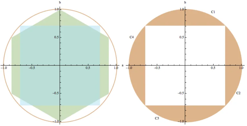
2.1 Mixed-Integer constraints applied to the determinant of Co(SO(2)). On the left, we illustrate square or hexagonal regions that are inadmissible for the variables in the rotation R ∈ Co(SO(2)). The resulting admis-sible regions are a union of individually convex sets, illustrated in the right as C1, . . . , C4 for the square region. . . 17

3.1 Momentum wheel [3] . . . 21

3.2 x, ytrajectory of spacecraft with momentum wheel using a Pd controller. The trajectory begins at (x, y) = (0,0) and ends at (10,10). . . 22

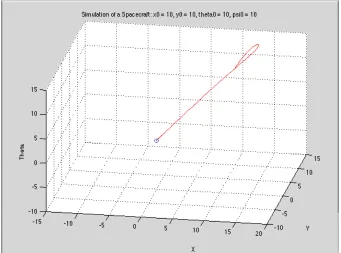
3.3 x, y, θ trajectory of spacecraft with momentum wheel using a Pd con-troller. . . 22

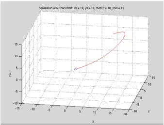
3.4 x, y, ψ trajectory of spacecraft with momentum wheel using a Pd con-troller. . . 23

3.5 Transfer orbit of a rocket from Earth to Mars [15] . . . 24

3.7 Trajectory for a 3D spacecraft maneuever is shown on the left. On the right is the determinant of the rotational state over the course of the maneuver. . . 25 3.8 Trajectory data for the 3D spacecraft maneuver. . . 26 3.9 UAV skyhook recapture system [16] . . . 28 3.10 Trajectory of an aerial vehicle using the Dubins car model. The

trajec-tory begins at (x, y) = (0,0) marked in green and ends at (5,10) marked in red. . . 29 3.11 Determinant of the rotation matrix R of an aerial vehicle using the

Dubins car model. . . 30 3.12 Trajectory of an aerial vehicle using a receding time horizon scheme

with CMPC at time t= 3. The green line marks the planned path and the blue line marks the path already traveled. The red dot signifies the vehicle’s current position. . . 32 3.13 Final trajectory of an aerial vehicle using a receding time horizon model

with CMPC. The vehicle starts at (x, y) = (0,0) and ends its trajectory at (5,10). . . 32 3.14 Example trajectory for the UAV when performing retrieval via

intercep-tion with rope locaintercep-tion. . . 35 3.15 Trajectory of an aerial vehicle using model predictive control. The

3.17 Total CPU time of CMPC using the Dubins car model over 1000 runs. 38

3.18 Optimal values of the MPC method over 1000 runs with heavy outliers thrown out. . . 38

3.19 Optimal values of the convex relaxation method using the Dubins car model over 1000 runs. . . 39

3.20 Ratio of MPC optimal value to Dubins optimal value over the subset of 1000 runs with ratios ≤10. . . 39 3.21 Increased performance of Dubins over MPC for the subset of 1000 runs

with Dubins ≤100% better. . . 40 3.22 Trajectory generated by MPC method incorporating obstacle avoiding

mixed integer constraints. The vehicle begins at (x, y) = (0,0) and stops at the goal (5, 10). . . 41

3.23 Trajectory generated by CMPC incorporating obstacle-avoiding Mixed-Integer constraints for both a physical obstacle and a convex hull ob-stacle. The vehicle begins at (x, y) = (0,0) and stops at the goal (5, 10). . . 42

3.24 Example trajectories for the Dubins car with and without a minimum speed of det(R) = 1₂, corresponding to the right of Figure 2.1. The trajectory begins at the origin and ends at (x, y) = (5,10). . . 42

1 Introduction

1.1

Objective

1.2

Motivation & Background

Motion planning is required whenever a robotic system, such as a rover or robotic arm, needs to make decisions about moving in an unknown environment [10]. The focus of this thesis is on the motion planning of two specific systems: spacecraft and unmanned aerial vehicles (UAVs). Free flying spacecraft need to be energy efficient when planning their navigation routes because they can only carry a limited supply of fuel. With more efficient motion planning algorithms, spacecraft will be able to travel farther to reaches of space never explored before. Furthermore, spacecraft, which for the most part do not currently have a high level of autonomy, will not have to rely as much on navigation routes sent from Earth, saving valuable time and resources. Similarly, if UAVs could compute their own navigational routes more efficiently, they could stay in the air and be active for longer periods of time. Specifically, if a plane can be easily collected with minimal damage, it can be reused for a different mission with little difficulty. The recapture technique we will be investigating involves having a UAV use a hook to latch onto a rope. The UAV will generate a trajectory to fly into the rope, latch on, and slide down for collection. This recapture method has recently gathered the interest of the U.S. Navy as well as several defense and aerospace companies.

cur-rent methods often require linearizing large amounts of data and as a result introduce not only approximation error in the dynamics, but also significant computing costs. Inspired by recent developments in convex optimization, a new technique has been developed [9] that does not require a large amount of input to produce a solution.

1.3

Explicit Model Predictive Control

A widely used method to control spacecraft is explicit model predictive control (MPC) [8]. This method has historically been popular in industry for process control. In this method, the system decides which path to take by minimizing a user-chosen cost while the current state of the system provides continual feedback. If the system is linear, it takes the form

s(k+ 1) =As(k) +Bu(k)

y(k) = Cs(k), (1.1)

where at time k, s(k) is the state of the system, u(k) is the input, and y(k) is the regulated output.

each time sample to change the problem into the linear form shown in 1.1. Oftentimes, MPC uses a receding time horizon scheme where it plans for a short period of time. It then executes one step of the optimization and repeats the planning calculation until time runs out. A particular advantage of this method is its ability to constantly readjust to changes in the environment that might affect the generated trajectory. However, the need to start a new optimization at each time step slows down the planning process considerably. Where our work differs is in our use of the convex hull ofSE(2) andSE(3) to constrain the motion of the system, which had previously required an infinite number of Linear Program constraints and thus has only been approximated.

Although MPC works well on many different and complex systems, linearization for complex systems may require significant computation and approximation. With the addition of many joints and robotic arms on spacecraft or with more complicated aerial vehicles like a quadrotor, the motion planning problem can be sufficiently com-plex to prevent the use of MPC for highly dynamic systems. Furthermore, due to the nature of the method, MPC does not guarantee a global minimum solution, only achieving a local minimum due to its local linearization.

1.4

Convex Optimization and Programming

motion planning of vehicular systems can be represented by a convex optimization problem, the computing power currently needed for vehicular control can be drasti-cally reduced. Convex functions can be defined as functions that satisfy the inequality

f(θu+ (1−θ)v)≤θf(u) + (1−θ)f(v), (1.2)

where f is a convex set, u, v ∈f, and 0≤θ ≤1. This definition often simplifies to:

∇2

f 0. (1.3)

as follows

min.f(x) (objective function)

such that gi(x)≤0, i= 1, . . . , m (inequality constraint)

aix=bi, i= 1, . . . , n (equality constraint). (1.4)

Thus, the solution x∗ would satisfy:

f(x∗) = inf{f(x)|gi(x)≤0, i= 1, . . . , m, aix=bi, i= 1, ..., n}. (1.5)

1.4.1

Convex Relaxation

The algorithm presented in this work relies on the use of orbitopes, the convex set consisting of convex hulls of the orbits given by a compact, algebraic group Gacting linearly on a real vector space. The convex hull conv(S) is the set of all convex combinations of points in S. More specifically, this method deals with a group acting on its identity element, or thetautological orbitope. It relaxes the constraint onSO(2), a rotation in 2 dimensions, from a unit sphere,p2_+q2 _{= 1, to a unit disk,p}2_+q2 _≤1

(LMI) [9] as follows

conv(SO(2)) ={



  

a b

−b a



  

:a2+b2 ≤1}

={     a b

−b a

    :         I     a b     a b 1        

0}. (1.6)

LMIs are a class of convex constraints that have had a profound effect on the field of optimization and control in recent decades [1], [2]. If the traditional motion planning problem can be formulated into a convex objective or cost function, the tautological orbitope LMIs can be applied as convex restraints to transform the problem into a semidefinite optimization problem.

1.5

Further Applications

2 Methodology

2.1

Analytical Methods

2.1.1

Rigid Body Transformations in

SE

(2) and

SE

(3)

In this work, the systems analyzed were assumed to act as rigid bodies, meaning that the distance between any two points on the body remains the same regardless of external forces. Therefore, when modeling the dynamics of a vehicle, rigid body transformations must be applied. These transformations are elements in SE(2) and SE(3) [11] containing the rotation (R) and translation (T) of the system at time t. In SE(2), the state of the system is as follows, withx, y representing the translation of the system and θ representing the orientation of the system

D=     R T 0 1     (2.1) D=        

cos θ −sin θ x sin θ cos θ y

0 0 1

        .

follows

R3 =

       

cosθ −sinθ 0 sinθ cosθ 0

0 0 1

        . (2.2)

2.1.2

MATLAB CVX

The MATLAB package CVX was used to solve the convex optimization problems formulated for motion planning simulations. The package uses a disciplined convex programming approach, and can also be used for geometric programming. With this approach, a basic library of convex functions and a small set of rules from convex analysis are used to solve the convex optimization problem. The problems involving mixed integer linear programming were numerically solved using MOSEK through CVX because the default CVX solver cannot support Mixed-Integer variables [6].

2.2

Experimental Methods

2.2.1

Ode45 Accuracy

other differential equation solvers. To test ode45, the function was implemented for a simple model two separate times. The first time,ode45 was implemented to generate a trajectory for a full time horizon. The second time, the function was applied every few seconds, using the result from the previous few seconds as the input for the next differential equation. The point at which the results differed between the two tests indicated the limits of ode45.

2.2.2

Pd Controller

A proportional-derivative (Pd) controller was applied to a spacecraft system to verify the dynamics of the vehicle. The control input, u, was set to be dependent on the state of the system,x

u=−Kx (2.3)

K =            

Kpx 0 0 0 Kvx 0 0 0

0 Kpy 0 0 0 Kvy 0 0

0 0 Kpθ 0 0 0 Kvθ 0

0 0 0 Kpψ 0 0 0 Kvψ

            , (2.4)

trajectory of the system from an initial position of disturbance to the origin.

2.3

Convex Model Predictive Control Over

SO(n)

We are concerned with the finite horizon control of systems which have a set of states R(t) that are restricted to lie in the special orthogonal group representing rotational

matrices, i.e. R(t) ∈ SO(n). We will furthermore assume that the dynamics of the system are linear with respect to this variable. For the remainder of this work, we will in particular consider systems where R(t) consists of the body orientation and forward velocity or acceleration in this body frame. Specifically, we use models of the form

˙

R(t) = AR(t) +Bu(t) (2.5) ˙

s(t) = R(t)M, (2.6)

where M is a fixed forward velocity vector in the body frame such as

M =         I     1 0     0 1         . (2.7)

We discretize such systems in time, and place them in the MPC framework, yield-ing optimizations of the followyield-ing form.

min. T

X

t=1

l(s(t), u(t)) +φ(x(T)) s.t. R(t+ 1) =R(t) +hu(t)

s(t+ 1) =R(t)·M

R(t)∈SO(n), (2.8)

where n= 2,3, and M is some forward vector in the body frame.

Via orbitopes, equation (2.8) is replaced with the convex constraintR(t)∈Co (SE(n)). The question then arises: under what scenarios will this relaxation be exact, i.e. when will the solution to the relaxed and original problems coincide? In related work [9], it was demonstrated that such a guarantee may be provided for a wide variety of computer vision problems. Unfortunately, no such guarantee is available in the MPC context. Instead, we propose optional non-convex restrictions on the variable R(t) based on Mixed-Integer constraints.

Systems with second-order dynamics on the rotation componentR(t) are handled in a similar fashion, with the simple addition of a state variable, for instance a variable

˙

2.3.1

Receding Time Horizon Control

Since motion planning involves movement in the future, all planning and control techniques need to handle some uncertainty. This uncertainty could come from in-strumentation, a changing environment, simplifying assumptions made in the model, or limitations in software or hardware accuracy. Planning entire trajectories and mis-sions at once saves computing time. However, the further the actions are planned to happen in the future, the more uncertainty measures will compound and propagate. Additionally, changes in the environment or other variables may require the model to be adjusted midway through the planned trajectory. To address these issues, a re-ceding time horizon control scheme was incorporated into some of the examples. The total time horizon remained at the same, but at each time step, the vehicle would plan a trajectory for a few time steps into the future and execute its planned movement for only one time step. Using this method, the vehicle begins a new optimization at each time step, dramatically increasing the number of optimizations calculated during one mission.

Because the trajectory was only planned a few time steps ahead, the vehicle could not be expected to reach its final destination in each of its planning steps. Instead of constraining the final position of the system to a chosen goal point, a penalty was put on the end condition. The penalty took the form

whereQis a diagonal matrix,x(t) is thex, yposition of the vehicle at timet, andx(tf) is the position of the vehicle at the end of the total time horizon. This penalty on the systems end condition was placed in the objective function of the convex optimization scheme.

2.3.2

Mixed-Integer Linear Programming (MILP)

MILP is a modification of a linear program (LP) in which some of the constraints take only integer values. For our purposes, the constraints will only take binary values, 0 or 1. MILP allows for the inclusion of discrete decisions, which are non-convex in the optimization problem. For instance, integer constraints enable capabilities such as obstacle avoidance in which a vehicle must determine whether to go ”left” or ”right” around an obstacle. By definition, MILP optimization problems are linear, so they will always output a globally optimal solution. In general, MILPs are nondeterministic polynomial time (NP)-complete [5], but in many cases they can be solved by relaxation to their LP form.

We review the encoding of obstacle avoidance into MILP constraints following [12]. For the two dimensional case with a rectangular obstacle, (xmin, ymin) is defined

as the lower left-hand corner of the obstacle and (xmax, ymax) is defined as the upper

right-hand corner of the obstacle. Points on the path of the vehicle (x, y) must lie outside of the obstacle, which can be formulated as a set of rectangular constraints. To convert these conditions to Mixed-Integer form, we introduce an arbitrary positive number M that is larger than any other variable in the problem. We also introduce integer variables ak that take values 0 or 1. The rectangular constraints now take the form

x≤xmin+M a1, (2.10)

−x≤ −xmax+M a2,

y≤ymin+M a3,

−y≤ −ymax+M a4, 4

X

k=1

ak ≤3.

Note that if ak = 1, then the kth constraint from (2.10) is relaxed. If ak = 0, then the kth _{constraint is enforced. The final MILP constraint ensures that at least one}

2.3.3

Convex Hull MILP Constraints

To use MILP to constrain solutions within the convex hull of SO(2), an ”obstacle” is introduced into the convex hull of SO(2). The hull of SO(2), as has been shown, can be represented as a circle of radius 1 centered at the origin, and the obstacle corresponds to a region within it that is admissible, preventing the determinant from obtaining a set of values. This is of importance as the forward velocity vector in the world frame is dependent on the forward velocity in the body frame, M in (2.8), rotated by R. Thus, a decrease in the determinant of R corresponds to a lower velocity, and a slowing of the vehicle. While appropriate in some contexts, e.g. land vehicles, it is undesirable in others, such as aircraft.

Ideally, this obstacle would be a circle that restricts the determinant of R from reaching 0. However, MILP constraints cannot represent a circular obstacle, so we start with a square obstacle by using the same form of constraints shown in (2.10). Illustrations of the determinant constraint are shown in Figure 2.1. As the number of faces is increased, the symmetry of the minimum speed constraint may be improved as desired.

2.3.4

Sources of Error

3 Results

3.1

Simple Satellite

For this experiment, a simple satellite experiencing constant thruster forces in the x, y,and θ directions were modeled in state space form. The MATLAB function

ode45 was applied to the model from time t= 0 to t=tf with the satellite starting

at the origin with 0 velocity. Then, ode45 was applied to the same model except at time t = 10, the position and velocity of the spacecraft were taken and used as the initial condition inputs for ode45 from time t = 10 to time t = 20. The process was repeated every 10 seconds until time t = tf. With this example, ode45 was found to be accurate for up to 670 seconds. At times after 670 seconds, the finite arithmetic errors of Matlab began to affect the results non-trivially. Fortunately, all the experiments performed in this thesis deal with time horizons less than 100 seconds, so the uncertainty propagation through the usage ofode45 for these purposes is negligible.

3.2

Spacecraft with Momentum Wheel

electric motor changes the rotational speed of the momentum wheel, the spacecraft begins to rotate in the opposite direction due to conservation of angular momentum. The spacecraft was once again subjected to constant thruster forces and a constant torque was applied to the momentum wheel. The mass of the satellite was arbitrarily set to five times the mass of the wheel.

Figure 3.1: Momentum wheel [3]

Figure 3.2: x, y trajectory of spacecraft with momentum wheel using a Pd controller. The trajectory begins at (x, y) = (0,0) and ends at (10,10).

Figure 3.4: x, y, ψ trajectory of spacecraft with momentum wheel using a Pd con-troller.

3.3

Transfer Orbits

The simple motion planning problem of transfer orbits was used as a starting point for the convex optimization experiments and simulations. In this problem, a spacecraft moves from one orbit to another (3.5).

Figure 3.5: Transfer orbit of a rocket from Earth to Mars [15]

was modeled by a rigid body transformation.

For this simulation, the initial orbit was set to x, y coordinates of (10, 10) and the final orbit was set to (0, 0). An initial velocity was set to the x and y velocity (0.5, 0) and the spacecraft was constrained to have a final velocity of (0, 0). A trajectory was successfully generated as shown in Figure 3.6 with a total CPU time of about 2.10 seconds and an optimal value of 1.82192e-05. The optimal value shows that the trajectory generated through convex relaxation requires very little energy. In addition, the curving at the beginning of the trajectory suggests that in this model, maintaining high speeds with a wider curvature is more energy efficient than minimizing path curvature.

of the trajectory, largely allowing the spacecraft to coast and conserve fuel.

0 2 4 6 8 10 12

0 1 2 3 4 5 6 7 8 9 10

Trajectory

X

Y

Figure 3.6: Trajectory of spacecraft between orbits using convex relaxation. The start point highlighted in green is at (10,10) and the goal point highlighted in red is (0,0).

Figure 3.8: Trajectory data for the 3D spacecraft maneuver.

3.4

Dubins Car Model

L(~q, ~u) =

Z tf

0

p

˙

x(t)2_{+ ˙y(t)}2_{dt, (3.1)}

wheretf is the time when the goal is reached, ˙x is the velocity in thex-direction, and ˙

y is the velocity in the y-direction. The configuration of the vehicle is designated by q= (x, y, θ). The solution of this Dubins path problem is given by

˙

x=Vcosθ ˙

y=Vsinθ ˙

θ =u, (3.2)

whereV is the constant speed of the vehicle anduis the turn rate [4]. The example on which we applied CMPC consisted of a UAV with no inertia attempting to latch onto a vertical rope for recapture as seen in Fig 3.9. Using a time horizon of 60 seconds, the UAV had its initial position set at the origin facing due north. The rope was set at a particular location, for instance at (5,10) where the distance was measured in feet. CMPC was implemented with the final position of the UAV constrained to equal the rope’s position at time t =tf.

Figure 3.9: UAV skyhook recapture system [16]

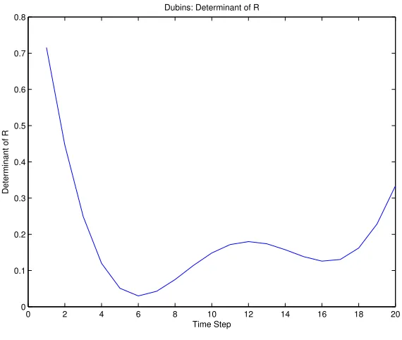
determinant of R should equal unity. In examining the determinant of the rotation matrix R we see that the convex relaxation is not always exact. Lower values of the determinant correspond to rotation matrices that lie inside the convex hull of SO(2), since the system is traveling at a velocity lower than maximum speed, v < V. As shown in Figure 3.11, the vehicle reaches top speed, then alternates slowing down and speeding up. The solution took approximately 0.1s to compute on a 2.3 GHz Intel i7 processor.

0 1 2 3 4 5 6

0 1 2 3 4 5 6 7 8 9 10

Dubins: Trajectory

X

Y

0 2 4 6 8 10 12 14 16 18 20 0

0.1 0.2 0.3 0.4 0.5 0.6 0.7 0.8

Dubins: Determinant of R

Time Step

Determinant of R

Figure 3.11: Determinant of the rotation matrix R of an aerial vehicle using the Dubins car model.

3.5

Receding Time Horizon

end condition (2.9).

As the condition det(R) = 0 corresponds to the UAV stopping altogether, phys-ically impossible for this application, we restrict det(R) > 0.3 using a MILP square constraint as detailed in the methods section. Each receding horizon iteration took approximately 0.16s to compute and the optimal value was 1.43268e-09. This exam-ple takes a larger amount of CPU time to compute because of the increased number of iterations. However, the increased amount of iterations allows for a more reliable, accurate, and efficient solution as seen by the optimal value being significantly lower in this example than in others. The trajectory at time t = 3 is shown (Figure 3.12) to illustrate the planning performed at each time step. The green trajectory is the planned path and the blue line is the trajectory the vehicle has already travelled. The final trajectory generated is shown in Figure 3.13.

3.6

Receding Time Horizon Rope Interception

0 0.5 1 1.5 2 2.5 3 3.5 4 4.5 5 0 1 2 3 4 5 6 7 8 9 10

Time step t=3

X

Y

Figure 3.12: Trajectory of an aerial vehicle using a receding time horizon scheme with CMPC at timet = 3. The green line marks the planned path and the blue line marks the path already traveled. The red dot signifies the vehicle’s current position.

0 1 2 3 4 5 6

0 2 4 6 8 10 12 Trajectory X Y

solved in MATLAB using CVX. The rope’s motion was modeled as follows

˙

xr =Axcos(ωt) (3.3)

˙

yr =Aysin(ωt+ψ)

Figure 3.14: Example trajectory for the UAV when performing retrieval via intercep-tion with rope locaintercep-tion.

3.7

MPC

0 1 2 3 4 5 6 0

1 2 3 4 5 6 7 8 9 10

MPC: Trajectory

X

Y

Figure 3.15: Trajectory of an aerial vehicle using model predictive control. The trajectory begins at (x, y) = (0,0) and ends at (5, 10).

3.8

Comparison Between MPC and Convex

Re-laxation

convex relaxation method however, it took about 1.4 - 2.3 seconds to generate a trajectory on average and the optimal values ranged from 0 - 1.4. Therefore, both methods took about the same amount of computational time, but CMPC generated solutions about up to 10 times more efficient than the currently used MPC method.

1.4 1.6 1.8 2 2.2 2.4 2.6 2.8

0 10 20 30 40 50 60 70 80 90 100

CPU Time (sec)

Frequency

MPC − CPU Time

Figure 3.16: Total CPU time of the MPC method over 1000 runs.

1.4 1.6 1.8 2 2.2 2.4 2.6 2.8 0

10 20 30 40 50 60 70 80 90

CPU Time (sec)

Frequency

Dubins − CPU Time

Figure 3.17: Total CPU time of CMPC using the Dubins car model over 1000 runs.

0 10 20 30 40 50 60 70 80 90 100

0 100 200 300 400 500 600

Optimal Value

Frequency

MPC − Optimal Value, Outliers Thrown Out

0 0.2 0.4 0.6 0.8 1 1.2 1.4 0

20 40 60 80 100 120

Optimal Value

Frequency

Dubins − Optimal Value

Figure 3.19: Optimal values of the convex relaxation method using the Dubins car model over 1000 runs.

0 1 2 3 4 5 6 7 8 9 10

0 20 40 60 80 100 120 140 160

Ratio of MPC Optimal Value/Dubins Optimal Value

Frequency

Ratio of MPC Optimal Value/Dubins Optimal Value

0 10 20 30 40 50 60 70 80 90 100 0

10 20 30 40 50 60

Percent Better Optimal Value of Dubins

Frequency

Percent Better Optimal Value of Dubins

Figure 3.21: Increased performance of Dubins over MPC for the subset of 1000 runs with Dubins ≤100% better.

3.9

Mixed-Integer Linear Programming (MILP)

Mixed-Integer constraints were added to the receding time horizon example in or-der to incorporate obstacle avoidance capabilities into both the MPC and convex relaxation examples. For simplicity and testing purposes, the initial simulations were performed using simple, rectangular obstacles. In both the receding time horizon (Figure 3.23) and MPC (Figure 3.22) cases, the physical obstacle was successfully avoided by introducing Mixed-Integer constraints as detailed in (2.10).

mini-mum size on the determinant of R, also shown in the Figures 3.24 and 3.25. With the minimum speed constraint the solution took approximately one minute to compute on a 2.3GHz Intel i7 processor. The differences between enforcing a minimum speed and not including that restriction are shown in Figures 3.24 and 3.25. Introducing an obstacle in the convex hull of SO(2) works as expected. The red dashed line in Figure 3.25 shows that the determinant of R in the Dubins car model example was forced to stay above the designated speed of det(R) = 1₂.

0 0.5 1 1.5 2 2.5 3 3.5 4 4.5 5

0 1 2 3 4 5 6 7 8 9 10

Trajectory

X

Y

−4 −3 −2 −1 0 1 2 3 4 5 0

1 2 3 4 5 6 7 8 9 10

UAV: Trajectory

X

Y

Figure 3.23: Trajectory generated by CMPC incorporating obstacle-avoiding Mixed-Integer constraints for both a physical obstacle and a convex hull obstacle. The vehicle begins at (x, y) = (0,0) and stops at the goal (5, 10).

Figure 3.24: Example trajectories for the Dubins car with and without a minimum speed ofdet(R) = 1

2, corresponding to the right of Figure 2.1. The trajectory begins

Figure 3.25: Determinant of theSO(2) stateR for the Dubins car trajectories shown in Figure 3.24 with and without the determinant constraint.

constraints after about 5 hours. The program was terminated at this time, so the trajectory shown is a sub-optimal solution. However, the algorithm is shown to allow the satellite to avoid the spacecraft successfully.

−6 −4 −2 0 2 4 6 8 10 12 14

0 0.5 1 1.5 2 2.5 3 3.5 4 4.5 5

Trajectory

X

Y

Figure 3.26: Trajectory for a satellite docking on a spacecraft using Mixed-Integer constraints to avoid collision with the spaceship.

4 Conclusion

Bibliography

[1] S.P. Boyd, L. El Ghaoui, E. Feron, and V. Balakrishnan. Linear Matrix

In-equalities in System and Control Theory. Society for Industrial and Applied

Mathematics, 1997.

[2] S.P. Boyd and L. Vandenberghe. Convex optimization. Cambridge University Press, 2004.

[3] Nona Cheeks. Photo: A small, high-torque reaction/momentum wheel. http:

//ipp.gsfc.nasa.gov/ft_tech_reaction_moment_whl.shtm, November 2012.

[4] Lester E Dubins. On curves of minimal length with a constraint on average curva-ture, and with prescribed initial and terminal positions and tangents. American

Journal of mathematics, pages 497–516, 1957.

[5] Christodoulos A Floudas. Nonlinear and mixed-integer optimization:

fundamen-tals and applications. Marcombo, 1995.

[6] Michael Grant, Stephen Boyd, and Yinyu Ye. Cvx: Matlab software for disci-plined convex programming, 2008.

[7] Christopher D Hall, Panagiotis Tsiotras, and Haijun Shen. Tracking rigid body motion using thrusters and momentum wheels. Journal of the Astronautical

[8] Øyvind Hegrenæs, Jan T Gravdahl, and Petter Tøndel. Spacecraft attitude control using explicit model predictive control. Automatica, 2005.

[9] Matanya B Horowitz, Nikolai Matni, and Joel W Burdick. Convex relaxations of se (2) and se (3) for visual pose estimation. arXiv preprint arXiv:1401.3700, 2014.

[10] Jean-Claude Latombe. Robot Motion Planning. Springer, 1990.

[11] Richard M Murray, Zexiang Li, and Shankar Sastry.A Mathematical Introduction

to Robotic Manipulation. Boca Raton: CRC, 1994.

[12] Arthur Richards and Jonathan How. Mixed-integer programming for control. In

American Control Conference, 2005. Proceedings of the 2005, pages 2676–2683.

IEEE, 2005.

[13] Arthur Richards and Jonathan P How. Aircraft trajectory planning with col-lision avoidance using mixed integer linear programming. In American Control

Conference, 2002. Proceedings of the 2002, volume 3, pages 1936–1941. IEEE,

2002.

[14] L.-L. Show, Jyh Ching Juang, Chen-Tsung Lin, and Y.-W. Jan. Spacecraft Robust Attitude Tracking Design: Pid Control Approach. In Proceedings of the

2002 American Control Conference, pages 1360–1365, 2002.

[15] Photo: Interplanetary trajectories. http://www2.jpl.nasa.gov/basics/

[16] Photo: An unmanned aerial vehicle (uav) scan eagle lands in the skyhook for recovery on the flight deck aboard the amphibious assault ship uss saipan, 2006.

[17] John T-Y Wen and Kenneth Kreutz-Delgado. The attitude control problem.