On the lack of robustness of hydrologic models regarding water balance simulation: a diagnostic approach applied to three models of increasing complexity on 20 mountainous catchments

www.hydrol-earth-syst-sci.net/18/727/2014/ doi:10.5194/hess-18-727-2014

© Author(s) 2014. CC Attribution 3.0 License.

Hydrology and

Earth System

Sciences

On the lack of robustness of hydrologic models regarding water

balance simulation: a diagnostic approach applied to three models

of increasing complexity on 20 mountainous catchments

L. Coron1,2, V. Andréassian1, C. Perrin1, M. Bourqui2, and F. Hendrickx2

1_{Irstea (formerly Cemagref), UR HBAN, 1 rue Pierre-Gilles de Gennes, 92761 Antony, France} 2_{EDF R & D LNHE, 6 quai Watier, 78401 Chatou, France}

Correspondence to: L. Coron ([email protected])

Received: 22 August 2013 – Published in Hydrol. Earth Syst. Sci. Discuss.: 5 September 2013 Revised: 8 January 2014 – Accepted: 22 January 2014 – Published: 21 February 2014

Abstract. This paper investigates the robustness of rainfall–

runoff models when their parameters are transferred in time. More specifically, we propose an approach to diagnose their ability to simulate water balance on periods with differ-ent hydroclimatic characteristics. The testing procedure con-sists in a series of parameter calibrations over 10 yr periods and the systematic analysis of mean flow volume errors on long records. This procedure was applied to three conceptual models of increasing structural complexity over 20 moun-tainous catchments in southern France. The results showed that robustness problems are common. Errors on 10 yr mean flow volume were significant for all calibration periods and model structures. Various graphical and numerical tools were used to investigate these errors and unexpectedly strong sim-ilarities were found in the temporal evolutions of these vol-ume errors. We indeed showed that relative changes in sim-ulated mean flow between 10 yr periods can remain similar, regardless of the calibration period or the conceptual model used. Surprisingly, using longer records for parameters op-timisation or using a semi-distributed 19-parameter daily model instead of a simple 1-parameter annual formula did not provide significant improvements regarding these simu-lation errors on flow volumes. While the actual causes for these robustness problems can be manifold and are difficult to identify in each case, this work highlights that the trans-ferability of water balance adjustments made during calibra-tion can be poor, with potentially huge impacts in the case of studies in non-stationary conditions.

1 Introduction

1.1 Confidence and evaluation of rainfall–runoff

modelling in a changing climate

Whether or not climate stationarity is an appropriate concept, it is becoming increasingly difficult to consider that catch-ments are static environmental systems (Milly et al., 2008; Koutsoyiannis, 2011; Matalas, 2012; Muñz et al., 2013). The hydroclimatic conditions observed during historical periods cannot be easily considered as representative of other periods (historical or future). At the same time, hydrological mod-els are increasingly used for water resources management or risk assessment, often for future, and different, climatic con-ditions. To date, many unknowns remain concerning the ro-bustness of conceptual models in a changing climate.

conceptual models lack robustness when used in contrasted climate conditions.

Long historical records that include contrasted sub-periods are needed for evaluating models robustness. Indeed, pro-jections of future discharges under a changed climate can-not be compared to observations, by definition. The lack of model robustness is often measured through changes in root mean square error, Nash–Sutcliffe (NS) efficiency (Nash and Sutcliffe, 1970) or similar quadratic error criteria, between different periods. These criteria have the advantage of re-flecting the model efficiency on all simulated time steps and can even be used to build “model robustness criteria”, as dis-cussed by Coron et al. (2012). In several publications exam-ining this issue, the authors showed the existence of almost systematic biases on simulated volumes, depending on the transfer conditions for model parameters (see Vaze et al., 2010; Merz et al., 2011; Coron et al., 2012; Seiller et al., 2012). Solving the problems of incorrect water balance, sim-ulation requires further investigations and has motivated the study reported herein. They are particularly relevant in the context of climate change impact studies, where conditions are known to evolve but biases on simulated volumes are commonly considered constant for lack of true robustness assessment.

Moreover, in conceptual modelling, failure situations of parameter transfer often seem to be blamed for the overly simplistic model used or the inadequate calibration period chosen, without proper checking. However, schemes for sys-tematic model testing and comparison are valuable tools. They allow progress to be made on the evaluation of the mod-els’ suitability and also on the understanding of real-world hydrological system functioning (Seibert, 2001; Andréassian et al., 2009; Clark et al., 2011). International initiatives such as the Distributed Model Intercomparison Project (DMIP) (Smith et al., 2004, 2012), Model Parameter Estimation Ex-periment (MOPEX) (Schaake et al., 2006; Chahinian et al., 2006) and Hydrological Ensemble Prediction Experiment (HEPEX) (Schaake et al., 2007; Thielen et al., 2008) are good examples of the use of these testing schemes. We think that these types of evaluation approaches must be generalised and innovative strategies should be devised to make the best use of the long time series now available.

1.2 Scope of the paper

This paper deals with the evaluation of model robustness and was motivated by the recent findings on the difficulties for RR model parameters to reproduce water balances. We pro-pose a simple diagnostic approach to further investigate this question. Using long hydrological records, we tested the ca-pacity of three different models to simulate mean flows over series of successive 10 yr periods different from the calibra-tion one. Specifically, we aimed at evaluating the influence of the model complexity or the period used for parameter cali-bration on their capacity to simulate water balances.

This paper is organised as follows: the catchment set and models used are presented in the next section; the testing methodology and analysis techniques are discussed in Sect. 3 and the corresponding results provided in Sect. 4; and a general discussion and the overall conclusions are given in Sects. 5 and 6, respectively.

2 Catchments and models

2.1 Set of 20 French catchments

2.1.1 Data description

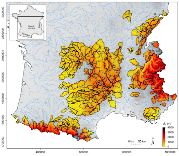
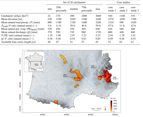
A set of 20 catchments was used to evaluate the robustness of hydrological models in their ability to simulate water bal-ances. These 20 catchments are located in southern France, mostly in mountainous areas (Massif Central, Pyrenees and French Alps, see Fig. 1). They cover a relatively wide range of characteristics, in terms of size, mean elevation, snow in-fluence and aridity index (see Table 1). The hydrological regimes are largely influenced by the processes of snow accu-mulation and melt for the most elevated catchments, and only governed by rainfall and evapotranspiration variations for the lowest ones. Three case studies were chosen to provide ex-amples of detailed results: the Ubaye River at Barcelonnette (case study 1), the Lot River at Barnassac (case study 2) and the Drac River at Pont de la Guinguette (case study 3). Case studies 1 and 3 are medium-size, high-elevation catchments located in the Alps. They have quite similar characteristics but marked differences in terms of precipitation. Case study 2 is a larger catchment in the Massif Central, with lower eleva-tion and consequently a much more limited snow influence.

Climate forcings and flow records were at least 40 yr, which cover a wide range of hydrometeorological conditions. Daily flow data were extracted from the HYDRO national archive (www.hydro.eaufrance.fr). They were checked for errors (by visual inspection and double mass curves analysis with neighbouring stations) and erroneous data were consid-ered as gaps. Total precipitation and air temperature series were extracted from the SPAZM reanalysis, which is based on ground network data and weather patterns. Developed by Gottardi et al. (2012), this reanalysis is available on 1×1 km cells at a daily time step from 1948 to 2010 for the main mountainous areas in France. These forcings can be consid-ered high-quality data. Finally, potential evapotranspiration (PE) time series were computed using either a Thornthwaite (1948) or Oudin et al. (2005) formula, depending on the model considered. In both cases, PE series were computed using air temperature from the SPAZM reanalysis.

2.1.2 Comments on the catchment selection process

Table 1. Characteristics of the 20-catchment set and the three case studies.

Set of 20 catchments Case studies

min 25th median 75th max case case case

percentile percentile study 1 study 2 study 3

Catchment surface[km2] 24 170 490 1000 3600 540 1160 510

Mean elevation[m] 520 1100 1650 2180 2440 2270 1050 1700

Mean annual total precip. (P)[mm] 880 1180 1320 1460 2260 1210 990 1620

Psolid/Pratio (annual mean)[−] 4 % 11 % 38 % 46 % 59 % 47 % 11 % 42 %

Mean annual pot. evap. (PEOudin)[mm] 330 430 470 560 640 410 560 460

Mean annual discharge (Q)[mm] 370 550 710 980 1720 600 440 860

P /PE ratio (annual mean)[−] 1.55 1.98 2.97 3.23 5.23 2.94 1.78 3.51

Q/P ratio (annual mean)[−] 0.36 0.48 0.54 0.63 0.85 0.49 0.44 0.53

Available time series length[yr] 40 47 51 57 62 52 62 42

Alps

Massif Central Pyrenees

@ @

@_@ case study 3

case study 1 a

a aa case study 2

Fig. 1. Locations of the 20 catchments used in this study.

When the catchment set used in this work was built, we attempted to neither exclude nor over-represent problematic situations. The availability of records of sufficient length and quality for our diagnostic approach mostly governed the se-lection procedure. Suspicious records were not kept and the catchments used here should be free of obvious quality prob-lems. Moreover, all the selected catchments are unregulated and are not particularly known for changes in their hydrolog-ical functioning for other reasons than climate variability.

The size of the catchment set was largely impacted by the demanding computation times for the calibration of the most complex model used in this work. From the initial database of 365 eligible catchments, 20 catchments were kept to pro-ceed with the full diagnostic approach. These catchments were also selected to be roughly representative of the va-riety of conditions in the initial database (although snow-dominated catchments are slightly over represented). The set

of 365 catchments was used to apply our testing procedure with the two simpler models, so as to confirm the findings presented here (the results can be found in the Appendix).

2.2 Three rainfall–runoff models of increasing

complexity – a “modelling transect”

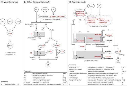
Three conceptual hydrological models were considered for this study and were chosen in order to cover a relatively wide range of structural complexity. Schematic diagrams of their structures are given in Fig. 2.

2.2.1 Mouelhi formula

Temp(X1 PE)

Temp(X2 PE)

D(max sun PE) f

P – SnowAcc.+ SnowMelt

Coeff(culture) ,

Index(permeability)

Hsoil,max

Hevap,soil

Hinfiltr.

Hsoil,inter

surface store:

Tsoil,high

Tsoil,low

Tinfiltr.

H gw,inter

groundwater store

Tgw,high

Tgw,low

Hevap,soil Pa(i-1)* PEa(i)*

Pa(i)*

Qa(i)*

* annual values for year i or i-1

PE

interception store

En

Pn-Ps Es

Pn

Ps

0.9 0.1

Q

X1

X3 f (X2)

Q1 Q9

Qd Qr

S

R Perc

f (X2) production

store

routing store

SH1(X4) SH2(X4)

P – SnowAcc.+ SnowMelt P Temp.

f (α)

Snow module: Kf (snow) Coeff (calor.) _{Snow module:}

D(max sun snow) Kf(snow)

Temp(snow) Temp(snow-melt)

Coeff(calor.) Temp(aging) AE

P Temp.

PE

f (c , D)

Q routing

a) Mouelhi formula b) GR4J-CemaNeige model c) Cequeau model

X1 production store capacity [mm]

X2 groundwater exchange coefficient [-]

X3 routing store capacity [mm]

X4 unit hydrograph time constant [day] Kf (snow) degree-day melt coefficient [mm.j-1] Coeff (calor.) weighting coefficient for snow pack thermal state [-]

Temp (X1/X2 PE) Thornthwaite PE parameter 1 / parameter 2 [°C]

D (max sun PE/snow) julian day of maximum PE / maximum snow [-]

Kf (snow) degree-day melt coefficient [mm.j-1_]

Temp (snow/snow-melt/aging) temperature threshold for snow- making/melt/aging [°C] Coeff (calor.) weighting coefficient for snow pack thermal state [-]

T infiltr./soil/gw time constant for filling or emptying of stores [d] H evap./infiltr./soil/gw max. capacity of stores or height threshold for emptying [mm]

c celerity coefficient for routing (1D Hayami) [d]

D diffusion coefficient for routing (1D Hayami) [d] α multiplication factor [-]

Parameters

Parameters

Parameters

Fig. 2. Structural schemes of the three models tested: (a) the Mouelhi formula, (b) GR4J-CemaNeige and (c) Cequeau (optimised parameters

are in red bold characters).

are cumulated annual precipitation and PE data (computed using Oudin’s formula). The model can be described using a non-linear equation:

Qa(j )=Pa(j )·



1−1/

"

1+

0.7·Pa(j )+0.3·Pa(j−1)

α·PEa(j )

2#0.5

,(1)

whereQa(j ),Pa(j )and PEa(j )are the annual discharge,

pre-cipitation and PE, respectively, for a given year (j), while

Pa(j−1) is the annual precipitation for the previous year

(j−1).

2.2.2 GR4J-CemaNeige model

GR4J is a parsimonious daily model with four calibrated pa-rameters, as described by Perrin et al. (2003). For this study, it is used with the CemaNeige degree-day type snow module developed by Valéry (2010). The required inputs for GR4J-CemaNeige are daily series for min/mean/max air tempera-ture, precipitation and PE (computed using Oudin’s formula). Both CemaNeige and GR4J are run at a daily time step. The snow module is computed over five elevation layers of equal surface and its outputs are then aggregated to feed GR4J,

which is a lumped model. The snow module has two free pa-rameters, which are optimised together with the four GR4J parameters.

2.2.3 Cequeau model

θ

θ

θ

θ

θ

θ

θ

θ

θ

θ

θ

θ

θ

θ

SP [01]

SP [02]

SP [03]

SP [04]

SP [05]

SP [06]

SP [07]

SP [08]

SP [09]

SP [10]

SP [11]

SP [12]

SP [13]

SP [14]

sub-period calibration

total period simulation

TP

TP

TP

TP

TP

TP

TP

TP

TP

TP

TP

TP

TP

TP

Fig. 3. Sub-period (SP) calibration procedure and simulation over the total period (TP) (example of 5 yr sub-periods within an 18 yr total

period).

2.2.4 Calibration procedure

Model parameters were calibrated by maximising the Kling– Gupta efficiency (KGE), proposed by Gupta et al. (2009). This criterion is given by

KGE=1− v u u

t_{ρ[Q,Q] −b 1}2+ σ[Q]b

σ[Q]−1

!2

+ µ[bQ]

µ[Q]−1

!2

, (2)

whereQandQbare the time series of observed and simulated

flow, respectively, at an annual time step for the Mouelhi for-mula and a daily time step for the GR4J-CemaNeige and Ce-queau models;ρ,σandµare the Pearson correlation coeffi-cient, the standard deviation and the mean, respectively.

Given the small number of free parameters for the Mouelhi formula and the GR4J-CemaNeige model, we used a sim-ple two-step calibration procedure: first the parameter space was screened using a gross predefined grid and the best pa-rameter set was then used as a starting point for a simple steepest ascent local search algorithm. This approach proved efficient for such parsimonious models compared to more complex search algorithms (Edijatno et al., 1999; Mathevet, 2005). The parameters from Cequeau were optimised using a more complex procedure developed by Le Moine (2009), which combines the multi-objective evolutionary annealing-simplex (MEAS) algorithm proposed by Efstratiadis and Koutsoyiannis (2005) and the multi-objective genetic algo-rithm,ε-NSGA-II, detailed by Reed and Devireddy (2004). This procedure has proved to be efficient in past applications of the Cequeau model for water resources assessment and dam management in France (Bourqui et al., 2011; François et al., 2013).

3 Robustness testing procedure

3.1 Subperiod calibration procedure

In a previous article, we proposed a testing methodol-ogy based on multiple transfer tests: the Generalised Split-Sample Test (GSST) procedure (Coron et al., 2012). It con-sists of a series of calibration-validation tests on indepen-dent sub-periods of equal length, considering all possible sub-period pairs. This testing procedure has been simplified for this study. The calibration sub-periods are built as in the GSST, i.e. using a sliding window that is moved by one hy-drological year between two neighbouring sub-periods (over-lap is allowed). However, we considered for this study a unique simulation period corresponding to the entire avail-able time series, contrary to what was done in the GSST. As a result, the calibration and simulation periods were not in-dependent and the transfer tests presented here should not be interpreted as strict split-sample tests. This testing procedure is illustrated in Fig. 3, whereθi is the optimal parameter set identified on the sub-periodi.

The testing procedure implemented in this work is highly dependent on the length of the sliding window used to build the calibration sub-periods. This length is chosen as a compromise, simultaneously allowing for correct parame-ter deparame-termination and a sufficient number of contrasted sub-periods. Here, we considered 10 yr calibration sub-periods (SP), while the available total periods (TP) were at least 40 yr and at most 62 yr for the catchment set (i.e. the number of sub-periods built per catchment ranged from 31 to 53).

Table 2. Model efficiencies computed over the total available records, considering sub-period calibrated parameter sets [KGETP]θSP.

Set of 20 catchments Case studies

min 25th median 75th max case case case

percentile percentile study 1 study 2 study 3

KGE at the annual time step

Mouelhi 0.048 0.572 0.760 0.883 0.942 0.899 0.713 0.919

GR4J-CemaNeige 0.497 0.814 0.871 0.905 0.968 0.868 0.883 0.896

Cequeau 0.277 0.810 0.881 0.921 0.971 0.884 0.898 0.901

KGE at the daily time step

GR4J-CemaNeige 0.670 0.828 0.866 0.899 0.943 0.864 0.848 0.838

Cequeau 0.724 0.845 0.878 0.902 0.943 0.890 0.881 0.876

were used for the time series split. Using hydrological instead of calendar years is important since some of the catchments considered in this work are snow-dominated (i.e. precipita-tions are stored as snow during the winter and only become runoff when spring arrives).

3.2 Model efficiencies

An overview of the model performances over the catchment set is provided in Table 2. For each catchment, KGE val-ues were computed over the total available record, consid-ering the various parameter sets stemming from our sub-period calibration procedure (see Fig. 3). For each model, the efficiencies were computed at the time step used to run the model, i.e. annual for the Mouelhi formula and daily for the GR4J-CemaNeige and Cequeau models. Additional KGE were computed at the annual time step for GR4J-CemaNeige and Cequeau (after series aggregation).

For these tests, the calibration periods (SP) are included in the simulation period (TP). The KGE values in Table 2 are therefore not exactly “validation” efficiencies. Still, they give a good idea of the models’ performances over the catchment set. On average, high efficiencies are reached for the daily models. Cequeau shows the highest criteria computed at both annual and daily time steps. The Mouelhi formula provides the lowest performances, but they remain acceptable on av-erage over the set.

3.3 Visual tools for robustness analysis

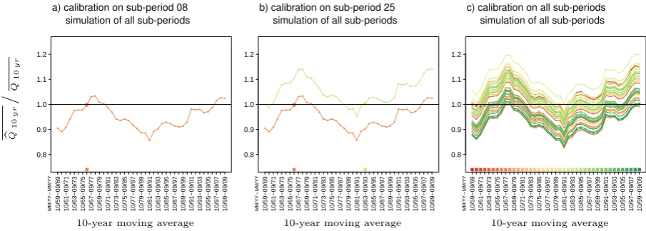
Previous studies on the temporal robustness of conceptual hydrological models have shown that volume errors can be significant as a result of parameter transfer (Merz et al., 2011; Coron et al., 2012). To further investigate this issue, we stud-ied the temporal variations of medium-term flow volume er-rors over the available records for different calibration con-figurations. These errors were expressed as a dimensionless bias given byQb10yr/Q10yr, in whichQb10yrandQ10yrare the 10 yr mean simulated and observed flows, respectively. The results obtained with different parameter sets can be super-imposed on the same graph. Thus, we built visual tools for analysing model behaviours. We illustrate their construction

with the example of the Ubaye River at Barcelonnette (case study 1 in Fig. 1), using the GR4J-CemaNeige model. Fig-ure 4 shows the successive steps followed to plot the varia-tions of mean flow volume errors.

Here, time series of precipitation, temperature and dis-charges were available over the 1959–2009 period. We built a total of 41 continuous sub-periods using a 10 yr sliding win-dow following the procedure presented in Fig. 3. These sub-periods were used to calibrate models and to compute vol-ume errors. The building procedure is explained is the next three subsections.

3.3.1 First step: using a single calibration period

(Fig. 4a)

Let us consider the example of sub-period SP[08] and plot the point corresponding to the errors in calibration (large cir-cle). Since volume errors are an important component of the calibration criteria (KGE), the mean flow volume error ob-tained for SP[08] was small (i.e. Qb10yr/Q10yr≈1). Then, from the simulated flows over the whole record using the cal-ibrated parameter set, we could compute the mean flow vol-ume error for each of the 40 remaining sub-periods and plot these errors for each of them (small dots). Note that there is an overlap between the calibration period and the neigh-bouring evaluation periods (for which the time lapse between starting years is less than nine years), but that the calibration and evaluation periods are independent in the other cases.

All 41 points were joined to form a curve, which is specific to the parameter set. This curve, notedωθSP[08], corresponds to

0.8 0.9 1.0 1.1 1.2 ● ● ● ● ●●● ● ●● ●● ● ● ● ●● ● ● ● ●● ● ●● ●●● ● ●● ● ●●● ●● ● ● ●● ●

10/59−09/69 10/61−09/71 10/63−09/73 10/65−09/75 10/67−09/77 10/69−09/79 10/71−09/81 10/73−09/83 10/75−09/85 10/77−09/87 10/79−09/89 10/81−09/91 10/83−09/93 10/85−09/95 10/87−09/97 10/89−09/99 10/91−09/01 10/93−09/03 10/95−09/05 10/97−09/07 10/99−09/09 a) calibration on sub-period 08

simulation of all sub-periods

b Q 10 y r

/

10-year moving average

MM/YY – MM/YY 0.8 0.9 1.0 1.1 1.2 ● ● ● ● ●●● ● ●● ●● ● ● ● ●● ● ● ● ●● ● ●● ●●● ● ●● ● ●●● ●● ● ● ●● ● ● ● ● ●●● ● ●● ●● ● ● ● ●●● ● ● ●● ● ● ● ●● ● ● ●● ● ●●● ●● ● ● ●● ● ●

10/59−09/69 10/61−09/71 10/63−09/73 10/65−09/75 10/67−09/77 10/69−09/79 10/71−09/81 10/73−09/83 10/75−09/85 10/77−09/87 10/79−09/89 10/81−09/91 10/83−09/93 10/85−09/95 10/87−09/97 10/89−09/99 10/91−09/01 10/93−09/03 10/95−09/05 10/97−09/07 10/99−09/09 b) calibration on sub-period 25

simulation of all sub-periods

10-year moving average

MM/YY – MM/YY 0.8 0.9 1.0 1.1 1.2 ● ● ● ● ●●● ● ●● ●● ● ● ● ●●● ● ● ●● ● ● ● ●● ● ●●● ● ● ●● ●● ● ● ●● ● ● ● ● ●●● ● ●● ●● ● ● ● ●● ● ● ● ●● ● ● ● ●●● ●●● ● ● ●● ●● ● ● ●● ● ● ● ● ●●● ● ●● ●● ● ● ● ●● ● ● ● ●● ● ●● ●● ● ●●● ● ●●● ●● ● ● ●● ● ● ● ● ●●● ● ●● ●● ● ● ● ●● ● ● ● ●● ● ● ● ●●● ●●● ● ●●● ●● ● ● ●● ● ● ● ● ●●● ● ●● ●● ● ● ●●● ● ● ● ●● ● ● ● ●●● ●●● ● ●●● ●● ● ● ●● ● ● ● ● ●●● ● ●● ●● ● ● ●●●● ● ● ●● ● ●● ●●● ●●● ● ●●● ●● ● ● ●● ● ● ● ● ●●● ● ●● ●● ● ● ●●●● ● ● ●● ● ● ● ●●● ●●● ● ●●● ●● ● ● ●● ● ● ● ● ●●● ● ●● ●● ● ● ● ●● ● ● ● ●● ● ●● ●●● ●●● ● ●●● ●● ● ● ●● ● ● ● ● ●●● ● ●● ●● ● ● ● ●● ● ● ● ●● ● ●● ●●● ● ●● ● ●●● ●● ● ● ●● ● ● ● ● ●●● ● ●● ●● ● ● ●●● ● ● ● ●● ● ● ● ●●● ●●● ● ●●● ●● ● ● ●● ● ● ● ● ●●● ● ●● ●● ● ● ● ●● ● ● ● ●● ● ●● ●●● ●●● ● ●●● ●● ● ● ●● ● ● ● ● ●●● ● ●● ●● ● ● ● ●● ● ● ● ●● ● ●● ●●● ●●● ● ●●● ●● ● ● ●● ● ● ● ● ●●● ● ●● ●● ● ● ●●●● ● ● ●● ● ● ● ●●● ●●● ● ●●● ●● ● ● ●● ● ● ● ● ●●● ● ●● ●● ● ● ● ●● ● ● ● ●● ● ● ● ●● ● ●●● ● ●●● ●● ● ● ●● ● ● ● ● ●●● ● ●● ●● ● ● ● ●● ● ● ● ●● ● ● ● ●●● ●●● ● ●●● ●● ● ● ●● ● ● ● ● ●●● ● ●● ●● ● ● ● ●● ● ● ● ●● ● ● ● ●●● ●●● ● ●●● ●● ● ● ●● ● ● ● ● ●●● ● ●● ● ● ● ● ●●●● ● ● ●● ● ●● ●●● ● ●● ● ●●● ●● ● ● ●● ● ● ● ● ●●● ● ●● ●● ● ● ● ●● ● ● ● ●● ● ● ● ●●● ● ●● ● ●●● ●● ● ● ●● ● ● ● ● ●●● ● ●● ●● ● ● ● ●●● ● ● ●● ● ● ● ●●● ●●● ● ● ●● ●● ● ● ●● ● ● ● ● ●●● ● ●● ● ● ● ● ● ●●● ● ● ●● ● ●● ●● ● ● ●● ● ●●● ●● ● ● ●● ● ● ● ● ●●● ● ●● ●● ● ● ● ●●● ● ● ●● ● ● ● ●● ● ● ●● ● ●●● ●● ● ● ●● ● ● ● ● ●●● ● ●● ● ● ● ● ● ●● ● ● ● ●● ● ● ● ●●● ●●● ● ●●● ●● ● ● ●● ● ● ● ● ●●● ● ●● ● ● ● ● ● ●● ● ● ● ●● ● ● ● ●●● ●●● ● ●●● ●● ● ● ●● ● ● ● ● ●●● ● ●● ●● ● ● ● ●● ● ● ● ●● ● ● ● ●● ● ● ●● ● ●●● ●● ● ● ●● ● ● ● ● ●●● ● ●● ●● ● ● ● ●● ● ● ● ●● ● ●● ●● ● ●●● ● ● ●● ●● ● ● ●● ● ● ● ● ●●● ● ●● ●● ● ● ● ●●● ● ● ●● ● ●● ●● ● ● ●● ● ●●● ●● ● ● ●● ● ● ● ● ●●● ● ●● ● ● ● ● ● ●● ● ● ● ●● ● ●● ●● ● ●●● ● ● ●● ●● ● ● ●● ● ● ● ● ●●● ● ●● ●● ● ● ● ●●● ● ● ●● ● ● ● ●● ● ●●● ● ● ●● ●● ● ● ●● ● ● ● ● ●●● ● ●● ●● ● ● ● ●●● ● ● ●● ● ● ● ●● ● ●●● ● ● ●● ●● ● ● ●● ● ● ● ● ●●● ● ●● ● ● ● ● ● ●●● ● ● ●● ● ●● ●●● ●●● ● ●●● ●● ● ● ●● ● ● ● ● ●●● ● ●● ●● ● ● ● ●●● ● ● ●● ● ●● ●●● ●●● ● ●●● ●● ● ● ●● ● ● ● ● ●●● ● ●● ●● ● ● ● ●●● ● ● ●● ● ●● ●● ● ●●● ● ●●● ●● ● ● ●● ● ● ● ● ●●● ● ●● ●● ● ● ●●●● ● ● ●● ● ●● ●●● ●●● ● ● ●● ●● ● ● ●● ● ● ● ● ●●● ● ●● ●● ● ● ● ●● ● ● ● ●● ● ●● ●● ● ●●● ● ●●● ●● ● ● ●● ● ● ● ● ●●● ● ●● ●● ● ● ● ●● ● ● ● ●● ● ● ● ●●● ●●● ● ● ●● ●● ● ● ●● ● ● ● ● ●●● ● ●● ●● ● ● ●●● ● ● ● ●● ● ● ● ●● ● ● ●● ● ●●● ●● ● ● ●● ● ● ● ● ●●● ● ●● ●● ● ● ●●●● ● ● ●● ● ●● ●● ● ●●● ● ● ●● ●● ● ● ●● ● ● ● ● ●●● ● ●● ●● ● ● ● ●● ● ● ● ●● ● ● ● ●● ● ●●● ● ●●● ●● ● ● ●● ● ● ● ● ●●● ● ●● ●● ● ● ●●●● ● ● ●● ● ●● ●●● ●●● ● ●●● ●● ● ● ●● ● ● ● ● ●●● ● ●● ●● ● ● ● ●● ● ● ● ●● ● ●● ●● ● ● ●● ● ●●● ●● ● ● ●● ● ● ● ● ●●● ● ●● ●● ● ● ●●● ● ● ● ●● ● ●● ●●● ●●● ● ●●● ●● ● ● ●● ●●●●●●●●●●●●●●●●●●●●●●●●●●●●●●●●●●●●●●●●●

10/59−09/69 10/61−09/71 10/63−09/73 10/65−09/75 10/67−09/77 10/69−09/79 10/71−09/81 10/73−09/83 10/75−09/85 10/77−09/87 10/79−09/89 10/81−09/91 10/83−09/93 10/85−09/95 10/87−09/97 10/89−09/99 10/91−09/01 10/93−09/03 10/95−09/05 10/97−09/07 10/99−09/09 c) calibration on all sub-periods

simulation of all sub-periods

10-year moving average

MM/YY

–

MM/YY

Fig. 4. Construction of the graphical representation of the series of 10 yr mean flow volume errors.

3.3.2 Second step: adding another calibration period

(Fig. 4b)

The previous step was repeated with a second calibration sub-period SP[25]. Again, mean flow volume errors were small for the calibration sub-period, but increased when the parameter set was transferred to simulate other parts of the time series. Interestingly, the shapes of theωθSP[08]andωθSP[25]

curves are similar, although their vertical positioning on the graph differs.

3.3.3 Last step: combining all calibration periods

(Fig. 4c)

This plotting procedure was used with all available parameter sets, i.e. considering all sub-periods as parameter “donors”. In each case, the entire time series was simulated and errors were computed on the 10 yr sub-periods. It can be noted that mean flow volume errors remain small during calibration in all cases and that the shapes of all the curves are similar, showing a “parallelism effect”.

3.3.4 Key questions

Numerous questions arose from the results obtained in the example of Fig. 4. First, each of the parallel curves illustrates a lack of robustness. A perfectly robust model would result in flat curves, i.e. the mean flow volume error would not depend on the period considered. Beyond noting alternating phases of 10 yr mean flow over- and underestimation, we then fo-cused on the following questions:

– The various parameter sets used to build Fig. 4c were

optimised over 10 yr. Are these calibration periods too short for the model to capture long-term dynamic pro-cesses? Would a calibration over the full record lead to correct volume simulations over the different parts of the time series?

– We observed behavioural similarities between

differ-ent parameter sets on the Ubaye River at Barcelon-nette. Are these similarities observed for other catch-ments from the set?

– Behavioural similarities were observed for

GR4J-CemaNeige. Are these similarities observed for sim-pler or more complex conceptual models?

3.4 Numerical criteria for analysis

Numerical criteria were built to measure the parameter trans-ferability issues in terms of volume errors and to assess the degree of similarity between series of mean flow volume er-rors obtained with different parameter sets. These criteria en-abled us to generalise our analyses over multiple catchments and models.

3.4.1 Measures of transferability

Since the focus here was on mean flow volume errors

(Qb10yr/Q10yr)and their temporal variations, we defined se-ries ofωθ curves as

ωθSP[i] =(uk)k∈[1:p]; uk =

h

b

QSP[k]

i

θSP[i]

QSP[k]

, (3)

where SP[i] and SP[k] are theith andkth 10 yr sub-periods chosen among theppossible ones;QSP[k] is the mean ob-served flow on SP[k] and[QbSP[k]]θSP[i]is the mean simulated

flow on SP[k] using the parameter set optimised on SP[i]. Computable for each hydrological model, these ωθSP[i]

curves reflect the extent of mean flow volume errors. They can be compared to assess the impact of changing the cali-bration sub-period on these errors (as shown in the example from Fig. 4). AnωθTP curve can be additionally considered

simulation period correspond to the total period (TP). Be-cause volume errors are an important component of the KGE calibration criterion, we expectωθTP to be the flattest of all theωθ curves. For this reason, we chose to consider theωθTP

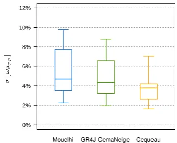
as a reference in the comparison criteria proposed hereafter. In order to measure the magnitude of the volume error temporal variations, we used the standard deviation opera-tor (σ) on theωθ curves. An example for the ωθTP curve is

given in Eq. (4):

σωθTP

=

v u u

t 1

p p X

k=1

(uk)2

!

− 1

p p X

k=1

(uk)

!2

;

uk =

h

b

QSP[k]

i

θTP

QSP[k]

(4) with the same notations as in Eq. (3).

This criterion reveals the overall ability for a model to re-produce 10 yr mean flow on various sub-periods when it is calibrated on the full available record. It varies between 0 (optimal situation with no errors) and+∞. The larger the values, the smaller the model transferability in time (at least with respect to mean flow volume errors).

3.4.2 Measures of behavioural similarity

Other criteria were designed to specifically address the ques-tion of behavioural similarity highlighted in Fig. 4c.

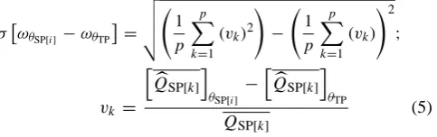
In line with the criterion of Eq. (4), the standard deviation operator was used again, but with a different objective this time: measuring the similarity betweenωθobtained from

dif-ferent parameter sets. The corresponding criterion is given in Eq. (5):

σ

ωθSP[i]−ωθTP

=

v u u

t 1

p

p

X

k=1

(vk)2

!

− 1

p

p

X

k=1

(vk)

!2

;

vk =

h

b

QSP[k]

i

θSP[i]

−hQbSP[k]

i

θTP

QSP[k]

(5) with the same notations as for Eq. (3).

As opposed to the previous one, this criterion is not infor-mative on the transferability level of a model, but measures the degree of “parallelism” between twoωθ curves. It takes

values between 0 (situation where the shapes of the ωθSP[i]

andωθTP curves are rigorously identical) and+∞. We note

that, by construction, the mean flow volume error over the entire record ([QbTP]θSP[i]/QTP) has no impact on this second

criterion. In other words, only the shape similarities between theωθcurves are analysed, while their vertical spacing is left

out of consideration.

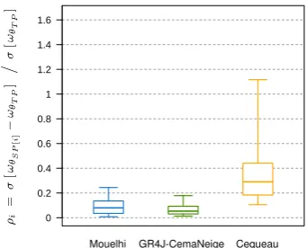
This measure of similarity was then normalised by the magnitude of volume error variations (σ[ωθTP]) to build a

non-dimensional criterion (ρi), given in Eq. (6). In a way,

ρi is a “noise-to-signal ratio” that highlights how similarωθ

curves are:

ρi =

σ

ωθSP[i] −ωθTP

σ

ωθTP

. (6)

Similarly, a criterion was built for inter-model compar-isons where the “degree of parallelism” on volume error vari-ations is measured between two models (M1andM2), both calibrated over the entire time series. Notedρ_M0

1M2, this

ra-tio, is described in Eq. (7) and corresponds to the compari-son between differentωθTP curves. The choice for the model

serving as reference, whose correspondingσ[ωθTP]

consti-tutes the denominator, is made arbitrarily:

ρ_M10 _M2 =

σhωM2_θTP −ω_θTPM1i

σhωM1_θTPi

. (7)

As for σ[ωθSP[i] −ωθTP], the criteria detailed in Eqs. (6)

and (7) range between 0 and+∞. The smaller theρi value,

the stronger the similarities between the ωθSP[i] and ωθTP

curves for the model considered. Similarly, the smaller the

ρ_M0

1M2 value, the stronger the similarities between theωθTP

curves from the models compared (M1andM2).

4 Results

4.1 Case studies: graphical analyses on three

catchments

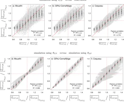
The graphical procedure illustrated in Fig. 4 was ap-plied to the 20 catchments and three hydrological mod-els described in Sect. 2.2 (the 1-parameter Mouelhi for-mula, the 6-parameter GR4J-CemaNeige model and the 19-parameter Cequeau model). Examples of results are given in Fig. 5 for three catchments: the Ubaye River at Barcelon-nette (540 km2, case study 1), the Lot River at Barnassac (1160 km2, case study 2) and the Drac River at Pont de la Guinguette (510 km2, case study 3). This figure is composed of 12 graphs, where the results obtained on the same catch-ment are in columns, while data and simulations with the same model are in rows. In all cases, we plotted the 10-yr moving average of the variables considered. For each graph showing simulation results, the grey curves correspond to the sub-period calibration procedure previously introduced (see Figs. 3 and 4), while the single black curve corresponds to the calibration over the entire record.

The graphs from Fig. 5 provide useful elements that help determine the impact of the calibration period on model robustness.