A global water scarcity assessment under Shared Socio economic Pathways – Part 2: Water availability and scarcity

(1)

Hydrol. Earth Syst. Sci., 17, 2393–2413, 2013 www.hydrol-earth-syst-sci.net/17/2393/2013/ doi:10.5194/hess-17-2393-2013

EGU Journal Logos (RGB)

Advances in

Geosciences

Open Access

Natural Hazards

and Earth System

Sciences

Open Access

Annales

Geophysicae

Open Access

Nonlinear Processes

in Geophysics

Open Access

Atmospheric

Chemistry

and Physics

Open Access

Atmospheric

Chemistry

and Physics

Open Access

Discussions

Atmospheric

Measurement

Techniques

Open Access

Atmospheric

Measurement

Techniques

Open Access

Discussions

Biogeosciences

Open Access Open Access

Biogeosciences

Discussions

Climate

of the Past

Climate

of the Past

Discussions

Earth System

Dynamics

Earth System

Dynamics

Discussions

Geoscientific

Instrumentation

Methods and

Data Systems

Open Access

_{Geoscientific}

Instrumentation

Methods and

Data Systems

Open Access

Discussions

Geoscientific

Model Development

Geoscientific

Model Development

Discussions

Hydrology and

Earth System

Sciences

Open Access

Hydrology and

Earth System

Sciences

Open Access

Discussions

Ocean Science

Discussions

Solid Earth

Discussions

The Cryosphere

Discussions

Natural Hazards

and Earth System

Sciences

Open Access

Discussions

A global water scarcity assessment under Shared Socio-economic

Pathways – Part 2: Water availability and scarcity

N. Hanasaki1, S. Fujimori1, T. Yamamoto2, S. Yoshikawa3, Y. Masaki1, Y. Hijioka1, M. Kainuma1, Y. Kanamori1, T. Masui1, K. Takahashi1, and S. Kanae3

1_{National Institute for Environmental Studies, Tsukuba, Japan} 2_{Nagaoka National College of Technology, Nagaoka, Japan} 3_{Tokyo Institute of Technology, Tokyo, Japan}

Correspondence to: N. Hanasaki ([email protected])

Received: 28 November 2012 – Published in Hydrol. Earth Syst. Sci. Discuss.: 18 December 2012 Revised: 8 May 2013 – Accepted: 9 May 2013 – Published: 1 July 2013

Abstract. A global water scarcity assessment for the 21st

century was conducted under the latest socio-economic scenario for global change studies, namely Shared Socio-economic Pathways (SSPs). SSPs depict five global situa-tions with substantially different socio-economic condisitua-tions. In the accompanying paper, a water use scenario compati-ble with the SSPs was developed. This scenario considers not only quantitative socio-economic factors such as pop-ulation and electricity production but also qualitative ones such as the degree of technological change and overall en-vironmental consciousness. In this paper, water availabil-ity and water scarcavailabil-ity were assessed using a global hydro-logical model called H08. H08 simulates both the natural water cycle and major human activities such as water ab-straction and reservoir operation. It simulates water avail-ability and use at daily time intervals at a spatial resolution of 0.5◦×0.5◦. A series of global hydrological simulations were conducted under the SSPs, taking into account differ-ent climate policy options and the results of climate models. Water scarcity was assessed using an index termed the Cu-mulative Abstraction to Demand ratio, which is expressed as the accumulation of daily water abstraction from a river divided by the daily consumption-based potential water de-mand. This index can be used to express whether renew-able water resources are availrenew-able from rivers when required. The results suggested that by 2071–2100 the population liv-ing under severely water-stressed conditions for SSP1-5 will reach 2588–2793×106(39–42 % of total population), 3966– 4298×106(46–50 %), 5334–5643×106(52–55 %), 3427– 3786×106(40–45 %), 3164–3379×106(46–49 %)

respec-tively, if climate policies are not adopted. Even in SSP1 (the scenario with least change in water use and climate) global water scarcity increases considerably, as compared to the present-day. This is mainly due to the growth in population and economic activity in developing countries, and partly due to hydrological changes induced by global warming.

1 Introduction

Water resources are essential to all societal and economic activities. Total global water use is increasing, mainly due to economic and population growth in developing countries (Shiklomanov, 2000; Vörösmarty et al., 2000; Oki et al., 2003; Oki and Kanae, 2006; Alcamo et al., 2007). Moreover, as a consequence of climate change, water availability is pro-jected to become restricted in many parts of the world from a hydrological perspective (Arnell, 1999, 2004; Kundzewitz et al., 2007; Döll, 2009).

(2)

Vuuren et al., 2011), and the climate scenario of the Coupled Model Intercomparison Project Phase 5 (CMIP5; Taylor et al., 2012). Second, we developed a water use scenario that is compatible with both the qualitative and quantitative aspects of the SSPs. Third, we assessed whether renewable water re-sources are available when they are needed at daily intervals. Our study is presented in a two-part paper. In the ac-companying paper (Hanasaki et al., 2013), we developed a water use scenario compatible with the five global situa-tions described in the SSPs. The scenario covers all of the 21st century at five year intervals, with a spatial resolution of 0.5◦×0.5◦. It includes five factors, namely, the irrigated area, crop intensity, irrigation efficiency, and withdrawal-based potential industrial and municipal water demands. In this paper we have conducted a series of numerical sim-ulations using a global water resources model called H08 (Hanasaki et al., 2008a, b). The model is able to simu-late both the natural water cycle and human water use to-gether with their interaction. The impact of different socio-economic conditions and climate change on water avail-ability and use were analyzed for various combinations of scenarios.

The structure of this paper is as follows. In Sect. 2, the models, input data and simulation settings are presented. The simulation results are discussed in Sects. 3 and 4. In Sect. 3, we analyzed the impact of climate change excluding socio-economic change. In Sect. 4 we analyzed the impact of both kinds of change. In Sect. 5, we summarize the key uncertain-ties in our study. In Sect. 6, we present our conclusions.

2 Materials and methods

2.1 Global water resources model H08

To estimate global water scarcity, we used the H08 global distributed hydrological model. A brief description of the H08 model is presented here, which is directly relevant to the results. A more detailed description is found in Hanasaki et al. (2006, 2008a, b).

H08 consists of six submodels, namely, land surface hy-drology, river routing, crop growth, reservoir operation, wa-ter abstraction, and environmental flow requirement. The land surface hydrology submodel is a single soil layer model solving both the surface energy and water balance. The river submodel is a single reservoir model assuming constant flow velocity. The crop growth submodel is a process-based crop model based on the formulation of the SWIM (Soil and Wa-ter Integrated Model) model (Krysanova et al., 2000). This submodel is used to estimate the crop calendar (e.g. plant-ing date, harvestplant-ing date and croppplant-ing period), which is es-sential to estimate the daily irrigation water requirement. Consumption-based potential irrigation water demand is de-fined as the irrigation water required to maintain soil mois-ture in the top 1 m of irrigated cropland at 75 % (100 % for

rice) during the cropping period. The reservoir operation sub-model determines the storage and release of 507 reservoirs worldwide with a storage capacity larger than 1.0×109m3 (Hanasaki et al., 2006). Each reservoir is individually located on the river map of H08. For reservoirs for which the primary purpose is irrigation water supply, the release is controlled to match the seasonal variation of consumption-based potential irrigation water demand in the lower reach. For reservoirs with other purposes, release and storage is controlled to min-imize seasonal and inter-annual variations in river flows, tak-ing into account the ratio of the storage capacity of reser-voirs and mean annual inflow. The environmental flow re-quirement submodel is a simple empirical model that esti-mates the amount of river discharge that should be kept in the channel to maintain the aquatic ecosystem. The model is based on case studies of regional practices, while the river discharge should ideally be unchanged for the preservation of the natural environment.

The water abstraction submodel abstracts water from rivers to meet the consumption-based potential water de-mand. Note that only consumptive water use is included and not return flow and delivery loss. Because the river submodel is relatively simple (see Oki et al., 1999 in detail), the flow velocity is not affected by water abstraction or environmen-tal flows. When large reservoirs are located in the upper stream, the river is affected by reservoir operation. H08 prior-itizes the simulation of municipal water abstraction, followed by industrial and irrigation water abstraction. Note that al-though Hanasaki et al. (2010) incorporated some additional subcomponents into H08, such as medium-sized reservoirs (reservoirs with storage capacity less than 1.0×109m3 ca-pacity) and non-local and non-renewable blue water (hypo-thetical water sources to close the balance of local water sup-ply and demand) they were excluded in this study because these terms include considerable uncertainties both in mod-eling and developing future scenarios. However, we did in-clude the 507 largest reservoirs, because they considerably affect the river discharge of the largest rivers in the world (Hanasaki et al., 2006; Haddeland et al., 2006). A schematic diagram of water abstraction is shown in Fig. 1.

(3)

River Agr (3)

Land grid cell

Large reservoirs 1km3_<

Ind (2)

[image:3.595.48.285.61.207.2]

Mun (1) Environmental flowrequirement is always left in the channel Irrigated cropland

Fig. 1. Schematic diagram of water abstraction in H08. Water is

only abstracted from rivers. A river is considered to be regulated if there are large reservoirs with a storage capacity of greater than 1.0×109m3. Water is abstracted to fulfill potential municipal, in-dustrial, and irrigation water demands on a daily basis. The environ-mental flow requirement (between 0–40 % of mean monthly river discharge) is always left in the river channel.

2.2 Meteorological data and scenarios

H08 requires the input of the eight meteorological variables listed in Table 1. For historical simulations, WATCH (Wa-ter and Global Change project) forcing data (Weedon et al., 2011; hereafter WFD) was used. WFD covers the whole globe at a 0.5×0.5◦spatial resolution. It covers the time pe-riod 1958–2001 at six-hourly intervals. We converted WFD into daily intervals, and used 1971–2000 as the base period.

For future simulations, the climate scenario of the CMIP5 was used. CMIP5 coordinates climate projections using global climate models (Taylor et al., 2012). As of Octo-ber 2012, the results of more than 40 global climate mod-els (GCMs) have been available via the internet. Although it is recommended to utilize all available GCMs to account for model uncertainty (Knutti et al., 2010), for practical rea-sons, we needed to restrict the number of GCMs used. We subjectively selected three GCMs, namely MIROC-ESM-CHEM (MIROC), HadGEM2-ES (HadGEM2), and GFDL-ESM2M (GFDL) (Table 2). There is an open discussion re-garding the selection of models (Knutti et al., 2010), but the models selected in this study are used in the Inter Sectoral Impact Model Intercomparison Project (ISI-MIP; http://www.isi-mip.org/), which enabled cross-checking with their results.

It is widely known that the output of GCMs contain sys-tematic biases. In this study, we corrected for the biases of air temperature, precipitation, and longwave downward radi-ation. Most of the earlier studies corrected only for air tem-perature and precipitation. We included longwave downward radiation, because this term shows an apparent increasing trend in all GCM projections. Moreover, this term is impor-tant in solving the surface energy balance. To remove bias, a

shifting and scaling methodology was used (e.g. Alcamo et al., 2007; Lehner et al., 2006).

T_ycor_,_m_,_d=T_yobs_,_m_,_d+Torg_future_,_m−Torg_baseline_,_m (1)

P_ycor_,_m_,_d=P_yobs_,_m_,_d×Porg_future_,_m÷Porg_baseline_,_m (2)

Lcor_y_,_m_,_d=Lobs_y_,_m_,_d×Lorg_future_,_m−Lorg_baseline_,_m, (3) whereT,P, andLdenote air temperature, precipitation, and longwave radiation, respectively. The superscripts cor, obs, and org denote bias-corrected, observation and original GCM values, respectively. The subscripts future, baseline y, m, d indicate future period, retrospective period, year, month, and day, respectively. The upper bar indicates that the mean of thirty years’ records has been taken. After correcting for tem-perature and precipitation, rainfall-snowfall separation was conducted following the method of Kondo (1994), which uses not only air temperature but also relative humidity.

2.3 Non-meteorological data and scenarios

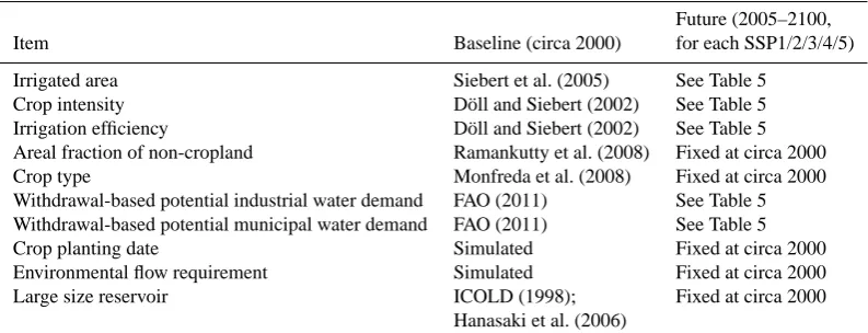
H08 requires the input of the non-meteorological variables listed in Table 3. For the other parameters of H08, we used the default values, as shown in Hanasaki et al. (2008a, b, 2010). For historical simulations, we used published datasets, which represent the period circa 2000. For future simula-tions, we used scenarios developed in the accompanying paper (Hanasaki et al., 2013) for the irrigated area, crop intensity, irrigation efficiency, and withdrawal-based poten-tial industrial and domestic water demand. Due to a lack of available information, the other variables were kept at present levels.

Crop type was set by using the crop type data of Mon-freda et al. (2008). They provided the areal fraction of 175 crop types, but we used only 19 that are commonly culti-vated worldwide. H08 is able to simulate up to two crops per year (multiple-cropping is common in the tropics), but needs to select only one crop type per grid cell during a cropping period (from planting to harvesting date). Here we assumed that the crop type of the largest fraction is planted in the first crop, and that of the second largest is in the second. We fixed the crop type throughout the 21st century, because of a lack of available data. This might be unrealistic because farmers would change the crop type to adapt to a changing climate and the demands of the crop. Because it is beyond the scope of this study to discuss future agricultural practices and food production, we left the crop type scenario until such time as the integrated assessment community can provide relevant scenarios and guidelines (see also the discussion in Sects. 3 and 6 of Hanasaki et al., 2013).

(4)

Table 1. Meteorological variables.

Item Baseline (1971–2000) Future

Rainfall [kg m−2s−1] Weedon et al. (2011) Scaling & separation (see text)

Snowfall [kg m−2s−1] Scaling & separation (see text)

Air temperature [K] Shifting (see text)

Longwave downward radiation [W m−2] Shifting (see text)

Shortwave downward radiation [W m−2] Fixed at present

Relative humidity [%] Fixed at present

Wind speed [m s−1] Fixed at present

Air pressure [Pa] Fixed at present

Table 2. Global climate models used in this study.

Modeling center Model name

Japan Agency for Marine-Earth Science and Technology, Atmosphere and Ocean Research Institute (University of Tokyo), and National Institute for Environmental Studies

MIROC-ESM-CHEM

Met Office Hadley Centre HadGEM2-ES

NOAA Geophysical Fluid Dynamics Laboratory GFDL-ESM2M

the factors 0.10 and 0.15 respectively, from the work of Shik-lomanov (2000). These values should be varied by country, time, and technological development. Because of a lack of information, we fixed these values throughout all countries, simulation periods, and scenarios. The values used could be too optimistic for developing countries with limited water re-cycling technology. Potential water demand for irrigation use is simulated by H08 as the consumption base. To convert this into the withdrawal base, which is used to calculate the With-drawal to Water Resources index explained below, we used the irrigation efficiency scenario developed in the accompa-nying paper (Hanasaki et al., 2013).

2.4 Simulation settings

We configured models and set up a simulation protocol as shown in Tables 4 and 5. We configured H08 in two forms, first for naturalized simulation (NAT), using only land sur-face and river submodels, and second for human simulation (HUM), using all six submodels. The NAT was used to as-sess a situation that assumed there was no human activity at all during the simulation periods, in order to evaluate the im-pact of climate change on the hydrological cycle. The HUM was used to assess water scarcity.

For the baseline period (1971–2000), two simulations were conducted with a naturalized configuration (NAT-Baseline) and human configuration (HUM-(NAT-Baseline).

For the future periods, we conducted four simulations: nat-uralized configuration (NAT-Future), human configuration fixing non-meteorological variables at circa 2000 (HUM-Fix), using the SSPs without a climate policy (business as usual; HUM-BAU), and using the SSPs with a climate

pol-icy (HUM-Polpol-icy). Three simulation periods were set, 2011– 2040, 2041–2070 and 2071–2100.

The NAT-Future simulation was conducted to analyze the hydrological response to climate change. H08 was set to a naturalized configuration, and future meteorological data (Eqs. 1–3) were prepared for three RCPs (RCP2.6, 4.5, 8.5) and three GCMs (MIROC, HadGEM2, GFDL).

The HUM-Fix simulation was conducted to analyze the magnitude of change in water availability and use due to climate change, excluding the effect of socio-economic changes. Three RCPs were used for three GCMs, but non-meteorological variables were fixed at the baseline period.

The HUM-BAU simulation was conducted to analyze wa-ter availability and scarcity under a business-as-usual situ-ation, with no climate policy. All five of the SSP scenarios were used. For each scenario, a RCP was selected that was compatible with the emission path as described in the ac-companying paper (Table 5, see also Fig. 3 of Hanasaki et al., 2013). Note that because the RCPs and SSPs have been developed independently, consistency between them is not strictly assured.

(5)

[image:5.595.99.496.82.234.2]

Table 3. Non-meteorological variables.

Future (2005–2100,

Item Baseline (circa 2000) for each SSP1/2/3/4/5)

Irrigated area Siebert et al. (2005) See Table 5

Crop intensity D¨oll and Siebert (2002) See Table 5

Irrigation efficiency D¨oll and Siebert (2002) See Table 5

Areal fraction of non-cropland Ramankutty et al. (2008) Fixed at circa 2000

Crop type Monfreda et al. (2008) Fixed at circa 2000

Withdrawal-based potential industrial water demand FAO (2011) See Table 5

Withdrawal-based potential municipal water demand FAO (2011) See Table 5

Crop planting date Simulated Fixed at circa 2000

Environmental flow requirement Simulated Fixed at circa 2000

Large size reservoir ICOLD (1998); Fixed at circa 2000

Hanasaki et al. (2006)

Table 4. Simulation settings.

Non-meteorological Emission Land and river Other

variables scenarios Period sub-models sub-models

NAT-Baseline 1971–2000 X

HUM-Baseline See Baseline of Table 3 1971–2000 X X

NAT-Future RCP2.6/4.5/8.5 2011–2040, 2041–2070, 2071–2100 X

HUM-Fix See Baseline of Table 3 RCP2.6/4.5/8.5 2011–2040, 2041–2070, 2071–2100 X X

HUM-BAU See Future of Table 3 See Table 5 2041–2070, 2071–2100 X X

HUM-Policy See Future of Table 3 See Table 5 2041–2070, 2071–2100 X X

2.5 Water scarcity index

Many earlier studies assessed water scarcity using an in-dex called the Withdrawal to Water Resources (WWR) ra-tio, which was devised by Raskin et al. (1997). The index expresses annual water withdrawal as a function of annual renewable water resources.

WWR=W/Q , (4)

whereQis the annual renewable water resource, typically substituted with mean annual river discharge [m3s−1] and

W is the annual total water withdrawal [m3s−1]. If water withdrawal exceeds 40 % of the water resources in a region, a chronic water shortage is indicated. This index is widely used, probably because it is intuitive and requires only two factors (W andQ) that are relatively easily available. How-ever, there are some well-known problems with the use of the WWR that are particularly important when it is applied to the assessment of climate change impacts. Climate change is projected to increase mean annual river discharges in many parts of the world, with an accompanying increase in the frequency and magnitude of the risk of floods and droughts (Kundzewitz et al., 2007). Because all of these variations are smoothed when the mean annual river discharge (i.e. the de-nominator of Eq. 4) is calculated, the WWR unintentionally underestimates these risks. A few studies have reported coun-termeasures. Wada et al. (2011) and Hoekstra et al. (2012)

computed the WWR on a monthly basis. Alcamo et al. (2007) proposed the consumption-to-Q90 ratio. Here“consumption” is the average monthly volume of water that is evaporated and “Q90” is a measure of the monthly river discharge that occurs under dry conditions (monthly discharge exceeds the Q90 value for 90 % of the time). These approaches success-fully identify the water scarcity in the most stressed month of the year, but do not easily determine water scarcity through-out the year as a whole. Hanasaki et al. (2008b) devised an index called the Cumulative Abstraction to Demand (CAD) ratio. The index was designed for modern global hydrologi-cal models, which can explicitly simulate the daily river dis-charge and water abstraction. This index is expressed as

CAD= 365 X

DOY=1 aDOY

, ₃₆₅

X

DOY=1

dDOY, (5)

whereaDOY anddDOY denote the simulated daily water

ab-straction from a river and the daily consumption-based po-tential water demand for a day of the year (DOY), respec-tively. If the accumulated water abstraction from the river (numerator) falls below the accumulated consumption-based potential water demand (denominator), water scarcity is in-dicated.aDOY≤dDOY can occur when a water source (i.e.

[image:5.595.51.548.276.374.2]

(6)

[image:6.595.53.544.94.269.2]

Table 5. Combination of SSPs and RCPs. See Table 5 of Hanasaki et al. (2013) for the scenario of irrigated area and crop intensity growth.

See Tables 6, 7, 8 of Hanasaki et al. (2013) for the improvement in efficiency of irrigation, industrial, and domestic water use, respectively.

Irrigated area Crop intensity Efficiency improvement Emission

Irrigation water use Industrial water use Domestic water use Scenario

SSP1 BAU Low Growth Low Growth High Efficiency High Efficiency High Efficiency RCP6.0

Policy RCP2.6

SSP2 BAU Medium Growth Medium Growth Medium Efficiency Medium Efficiency Medium Efficiency RCP8.5

Policy RCP4.5

SSP3 BAU High Growth High Growth Low Efficiency Low Efficiency Low Efficiency RCP8.5

Policy RCP6.0

SSP4 BAU Low Growth Low Growth Mixture of Efficiency Mixture of Efficiency Mixture of Efficiency RCP6.0

Policy RCP2.6

SSP5 BAU High Growth High Growth High Efficiency High Efficiency High Efficiency RCP8.5

Policy RCP6.0

This index is conceptual and for simulation only. In real-ity, not only river water but also groundwater, water stored in reservoirs and water diverted from different river basins are sources of water. In numerical simulations, all of these fac-tors can be disabled, allowing the relationship between the natural hydrological cycle and human-water demand to be analyzed. When the CAD falls below unity, it does not nec-essarily indicate that a region is experiencing a water short-age, but it does indicate the need for an alternative source of water other than natural river flow.

Hanasaki et al. (2008b) estimated the CAD globally us-ing the H08 water resources model. They identified regions that experience a gap in their subannual distribution of wa-ter availability and wawa-ter use, including the Sahel, the Asian monsoon region, and southern Africa. Due to the large con-trast between wet and dry seasons, these regions frequently suffer from seasonal water shortages in dry periods. They ret-rospectively assessed the period of 1986–1995, but not un-der climate change conditions. Thus, the CAD is used for a global change impact assessment on water scarcity for the first time in this study.

3 Results and discussion Part 1: impact of climate change

This section provides basic information regarding the re-sponse of hydrology and the water scarcity index to cli-mate change. Socio-economic change is excluded on pur-pose. Both climate and socio-economic change are consid-ered in the next section.

In this section, we analyze the results of the NAT-Future and HUM-Fix simulations and compare them with the NAT-Baseline and HUM-NAT-Baseline simulations, respectively. The results of the HUM-Baseline simulation are shown in Fig. 2. As can be seen from Table 4, non-meteorological data, such

as population and land use, was not used or fixed at the base-line period in these settings.

3.1 Climate change

First, we focus on the change in air temperature, which in-dicates the magnitude of climate change. We then consider the change in precipitation, which directly impacts water re-sources and consumption-based potential irrigation water de-mand.

Tables 6 and 7 show the changes in mean global terrestrial (i.e. land only excluding the Antarctica) temperature and pre-cipitation, respectively. The projected rise of global terres-trial mean temperature in 2071–2100, compared to the base-line period (1971–2000), was 1.2–2.4 K (RCP 2.6), 2.0–3.9 K (RCP 4.5), and 3.8–6.4 K (RCP 8.5). Global mean precipita-tion increased by 0.8–4.5, 1.9–5.9, and 3.6–9.5 %, respec-tively. The MIROC projection produced the largest increases among the three models. HadGEM2 projected a similar tem-perature rise to MIROC, but the change in precipitation was slightly smaller. GFDL projected the least change in both temperature and precipitation among the three models, being less than half of MIROC and HadGEM2.

(7)

(a)Temperature (b)Precipitation (c)Runoff

(d)Pot_Agri_Water_Demand (e)WWR (f)CWD

243 253 263 273 283 293 303 313 1 10 50 200 500 1000 3000 10000 1 10 50 200 500 1000 3000 1000

[image:7.595.87.511.64.237.2]

0.00 0.01 0.50 5.00 50.00 500.00 0.0 0.1 0.4 1.0 0.0 0.5 0.8 1.0

Fig. 2. Input and output of the HUM-Baseline simulation. (a) Air temperature [K], (b) precipitation [mm yr−1], (c) total runoff [mm yr−1],

(d) withdrawal-based potential irrigation water demand [m3s−1], (e) withdrawal to water resources ratio (WWR) [–], and (f) cumulative abstraction to demand ratio (CAD) [–]. Gray indicates missing values.

RCP2.6_2011−2040 RCP2.6_2041−2070 RCP2.6_2071−2100

RCP4.5_2011−2040 RCP4.5_2041−2070 RCP4.5_2071−2100

RCP8.5_2011−2040 RCP8.5_2041−2070 RCP8.5_2071−2100

0 2 4 6 8 10

Fig. 3. Global pattern of change (difference) in mean annual temperature from the baseline period [K].

increased rapidly, as compared to the low latitudes. Precipi-tation decreased in semi-arid areas such as near the Mediter-ranean Sea, central to western mid-latitude North America, southern Africa and southeastern South America. One im-portant finding, as shown by Tables 6–7 and Figs. 3–4 is that there is no clear difference when using RCP2.6, RCP4.5, and RCP8.5 in 2011–2040. There are distinct differences after 2041–2070 in terms of both the mean global changes and geographical patterns.

3.2 Hydrological change

Next, the change in mean estimated annual runoff is dis-cussed. Mean annual runoff is a key variable in the assess-ment of water resources, because it corresponds to regional renewable water resources. We focused on the results of the NAT-Future simulation, which displayed a hydrological response to climate change.

[image:7.595.85.512.290.545.2]

(8)

RCP2.6_2011−2040 RCP2.6_2041−2070 RCP2.6_2071−2100

RCP4.5_2011−2040 RCP4.5_2041−2070 RCP4.5_2071−2100

RCP8.5_2011−2040 RCP8.5_2041−2070 RCP8.5_2071−2100

[image:8.595.83.511.61.313.2]

0.0 0.5 0.9 1.1 1.5 2.0

Fig. 4. Global patterns of change (ratio) in the mean annual precipitation from the baseline period [–]. Regions shown in gray indicate that

the precipitation was less than 10 mm per month equivalent, and for this condition a precipitation bias correction was not applied (see text).

Table 6. Global terrestrial mean temperature change projected by the three GCMs. Baseline period (1971–2000) is 286.2 K.

RCP2.6 RCP4.5 RCP8.5

2011–2040 2041–2070 2071–2100 2011–2040 2041–2070 2071–2100 2011–2040 2041–2070 2071–2100

MIROC 1.7 K 2.4 K 2.4 K 1.5 K 2.9 K 3.6 K 1.7 K 3.8 K 6.3 K

HadGEM 1.8 K 2.4 K 2.3 K 1.7 K 3.1 K 3.9 K 1.9 K 4.0 K 6.4 K

GFDL 1.1 K 1.3 K 1.2 K 1.2 K 1.8 K 2.0 K 1.2 K 2.4 K 3.8 K

projected the largest increase in runoff among the three mod-els, which is consistent with the change in precipitation.

Figure 5 shows the geographical pattern of the change in runoff. Although the pattern of runoff changes (i.e. red-blue distribution) was similar to that of precipitation changes (Fig. 4), there was a much stronger contrast with the regional pattern (the color schemes are identical for Figs. 4 and 5). Generally, runoff increased in the northern high latitudes and decreased in the mid-latitudes. The figure indicates that, for MIROC under the RCP8.5 scenario, the mean annual runoff in 2071–2100 was altered by more than 10 % from the base-line period, in almost all regions of the world.

3.3 Withdrawal-based potential irrigation water demand

Next, the simulated withdrawal-based potential irrigation water demand is discussed using the results of HUM-Fix simulations. Table 9 shows the projected change in global to-tal withdrawal-based potential irrigation water demand. The projected ranges for RCP2.6, RCP4.5, and RCP8.5 were

−0.2–1.6, 1.9–2.8, and 6.7–10.0 %, respectively, in 2071– 2100. This indicates that the total global withdrawal-based potential irrigation water demand increases in almost all sce-narios. This is consistent with the findings of D¨oll (2002) who reported the results of similar numerical experiments. The difference among models and scenarios was small in 2011–2040, but became more distinct after 2041–2070.

[image:8.595.51.545.377.446.2]

(9)

[image:9.595.49.543.85.150.2]

Table 7. Global terrestrial mean precipitation change projected by the three GCMs. Baseline period (1971–2000) is 873 mm yr−1.

2011–2040 2041–2070 2071–2100 2011–2040 2041–2070 2071–2100 2011–2040 2041–2070 2071–2100

MIROC 2.3 % 4.8 % 4.5 % 2.4 % 4.8 % 5.9 % 2.5 % 6.0 % 9.5 %

HadGEM 2.1 % 2.9 % 3.4 % 2.4 % 3.8 % 5.2 % 2.5 % 4.1 % 4.3 %

[image:9.595.54.542.188.255.2]

GFDL 0.5 % 0.9 % 0.8 % 0.4 % 1.8 % 1.9 % 1.0 % 1.7 % 3.6 %

Table 8. Global mean runoff change projected by the three GCMs. Baseline period (1971–2000) is 407.6 mm yr−1.

2011–2040 2041–2070 2071–2100 2011–2040 2041–2070 2071–2100 2011–2040 2041–2070 2071–2100

MIROC 1.7 % 5.1 % 4.7 % 2.5 % 4.5 % 6.2 % 2.3 % 5.6 % 9.6 %

HadGEM 5.5 % 6.5 % 6.9 % 5.1 % 5.4 % 7.6 % 5.1 % 6.9 % 5.6 %

GFDL 0.9 % 0.3 % 1.1 % −0.4 % 2.8 % 3.1 % 1.5 % 2.3 % 4.3 %

the potential evapotranspiration, which eventually leads to a higher water requirement.

3.4 Withdrawal to water resources ratio

Water scarcity was assessed using the WWR. We focused on both the index itself (W/Q)and the so-called water-stressed population, which is defined here as the total population liv-ing in grid cells where the index exceeds 0.4.

Table 10 shows the total global water-stressed population and highlights two interesting findings. First, the estimated water-stressed population varied only marginally across all scenarios. Second, there was no clear relationship between the water-stressed population and either time or GHG emis-sions (i.e. RCPs). In some simulations, water stress decreased as time progressed (e.g. when using RCP2.6 in MIROC the water-stressed population in 2041–2070 was smaller than in 2011–2040) or as GHG emissions increased (e.g. in 2071– 2100 of MIROC, the water-stressed population using RCP4.5 was smaller than when using RCP2.6).

The minor changes in the water-stressed population can be primarily explained by the robustness of the index. In the HUM-Fix simulation, we fixed W (the numerator of Eq. 4). Irrigation water withdrawal was also affected by cli-mate change but the change was small. Therefore,Q (the denominator) had the primary role in this assessment. Al-though climate change affected the hydrological cycle glob-ally, it did not alter the spatial pattern of world climatic zones (i.e. fundamentally, the dry regions remained dry, and the wet regions remained wet). This prevented substantial change in the index. Consequently, densely populated grid cells where the index far exceeded 0.4 generated water-stressed popula-tion in all scenarios. The estimapopula-tion of the total global water-stressed population was considered to be robust due to these factors.

To analyze the change in the water-stressed population, we focused on the change in WWR. Figure 7 shows the

geo-graphical pattern of changes in the WWR. We defined the change as the ratio of WWR of the future period to the base-line, because WWR takes a wide range (almost zero in wet unpopulated regions to thousands in dry populated regions). The positive and negative signs basically correspond to the runoff scenario from Fig. 5. WWR increased where runoff decreased and vice versa. Note that the change was shifted toward the negative (i.e. water scarcity) direction, because global irrigation water withdrawal increased slightly (Fig. 6). Table 10 shows the population living in the grid cells where water stress conditions improved (WWR decreased) or worsened (WWR increased). Again, some interesting results were observed. Water stress conditions improved for more than half of the population for most of the cases shown in Ta-ble 10. This may indicate that climate change alleviates water scarcity or an increase in mean annual runoff may improve the availability of water. These issues are further investigated in the next subsection.

3.5 Cumulative abstraction to demand ratio

In order to further investigate water scarcity following cli-mate change, the CAD is used in this section. We focused on both the index itself and the water-stressed population, which is defined here as the total population living in a grid where the index falls below 0.5 (Hanasaki et al., 2008b).

Table 11 shows the projected water-stressed population. A clear relationship was observed where the stressed popula-tion increased over time and with increasing GHG emissions, i.e. climate change degraded water availability. However, as with the WWR results, the water-stressed population did not change significantly among scenarios. This is due to the same reasons we discussed in the previous subsection: regions with a strong seasonality in both water availability and use retain these features under various climate change scenarios.

(10)

[image:10.595.55.520.79.403.2]

Table 9. Global mean irrigation water withdrawal projected by the three GCMs. Baseline period (1971–2000) is 3214 km3yr−1.

2011–2040 2041–2070 2071–2100 2011–2040 2041–2070 2071–2100 2011–2040 2041–2070 2071–2100

MIROC 1.4 % 0.8 % 1.6 % 1.4 % 2.4 % 2.8 % 2.0 % 4.8 % 10.0 %

HadGEM 0.9 % −0.0 % −0.2 % 0.6 % 1.7 % 1.9 % 0.9 % 2.9 % 6.7 %

GFDL 1.8 % 2.0 % 1.1 % 2.3 % 2.3 % 2.4 % 1.7 % 3.8 % 7.1 %

RCP2.6_2011_2040 RCP2.6_2041_2070 RCP2.6_2071_2100

RCP4.5_2011_2040 RCP4.5_2041_2070 RCP4.5_2071_2100

RCP8.5_2011_2040 RCP8.5_2041_2070 RCP8.5_2071_2100

0.0 0.5 0.9 1.1 1.5 2.0

Fig. 5. Global pattern of change (ratio) in the mean annual runoff from the baseline period [–].

the water stress increased. The pattern differs from that of runoff change (Fig. 5), indicating that, although the total annual runoff increased, water resources were not available when they were needed. For example, while the mean an-nual runoff increased in the Sahel regions, CAD decreased (i.e. water stress increases). The increase in runoff in the wet seasons did not contribute to water resources in dry seasons, and the gap between water availability and use in dry seasons worsened. The results imply that the increase in mean annual runoff did not alleviate water scarcity in these regions.

Table 11 shows the population living in the grid cells where water stress conditions improved (CAD increased) or worsened (CAD decreased). The population suffered from an increase in water stress over time and with increased GHG emissions. Although total global runoff increased, the results indicate that less than 30 % of the population benefitted in terms of improved water availability.

The results using the CAD are substantially different from those using the WWR. The WWR has been widely used in previous water resource assessments, but the results should be interpreted with caution when it is applied to climate change impact assessments. Because of the nature of the WWR, water stress is alleviated when the mean annual runoff

increases. Mean annual runoff could be increased by rain-fall in a rainy season or under extreme precipitation. These increases are usually difficult to utilize as water resources (Kundzewitz et al., 2007). The CAD is expressed as the ac-cumulation of daily abstraction from rivers divided by the accumulation of daily consumption-based potential water de-mand. This index is useful for determining whether water is available when it is needed, taking into account the seasonal-ity of both water availabilseasonal-ity and use. Excess water (e.g. flood water in wet seasons) is not considered to be available, which is an advantage over WWR.

4 Results and discussion Part 2: impact of climate and socio-economic change

This section provides the results of the global water scarcity assessment regarding the response to climate and socio-economic change.

(11)

RCP2.6_2011−2040 RCP2.6_2041−2070 RCP2.6_2071−2100

RCP4.5_2011−2040 RCP4.5_2041−2070 RCP4.5_2071−2100

RCP8.5_2011−2040 RCP8.5_2041−2070 RCP8.5_2071−2100

[image:11.595.98.498.61.298.2]

0.0 0.5 0.9 1.1 1.5 2.0

[image:11.595.51.548.373.500.2]

Fig. 6. Global pattern of change (ratio) in the mean annual withdrawal-based irrigation water demand from the baseline period [–].

Table 10. Global total population living under the condition of WWR≥0.4, living where the index improved (WWR decreased), and living where the index worsened (WWR increased) (×106person). See text for the caveats used when interpreting if the index improved/worsened. The number in brackets is the percentage of the global total population. Baseline period (1971–2000) is 1716×106person.

2011–2040 2041–2070 2071–2100 2011–2040 2041–2070 2071–2100 2011–2040 2041–2070 2071–2100

MIROC Stressed 1678 (27) 1557 (25) 1641 (27) 1616 (26) 1612 (26) 1585 (26) 1700 (28) 1630 (26) 1722 (28) Improved 3306 (54) 4064 (67) 3730 (61) 3652 (60) 3826 (63) 3839 (63) 3143 (51) 3544 (58) 3135 (51) Worsened 2749 (45) 1991 (32) 2325 (38) 2403 (39) 2229 (36) 2217 (36) 2912 (48) 2512 (41) 2921 (48)

HadGEM2 Stressed 1549 (25) 1464 (24) 1487 (24) 1547 (25) 1571 (25) 1522 (25) 1553 (25) 1526 (25) 1548 (25) Improved 3929 (64) 4376 (72) 4491 (74) 4151 (68) 3940 (65) 4310 (71) 4071 (67) 3765 (62) 3811 (62) Worsened 2126 (35) 1679 (27) 1564 (25) 1904 (31) 2115 (34) 1746 (28) 1985 (32) 2291 (37) 2244 (37)

GFDL Stressed 1725 (28) 1711 (28) 1694 (27) 1750 (28) 1705 (28) 1683 (27) 1674 (27) 1739 (28) 1782 (29) Improved 3080 (50) 3173 (52) 3350 (55) 2565 (42) 2822 (46) 3459 (57) 3256 (53) 2949 (48) 2742 (45) Worsened 2975 (49) 2883 (47) 2706 (44) 3490 (57) 3233 (53) 2596 (42) 2799 (46) 3107 (51) 3313 (54)

assessed using the CAD. As discussed in Sects. 3.4 and 3.5, although WWR has been widely used in previous studies, it can be misleading when interpreting the impact of climate change on water scarcity. The results using the WWR are given in Appendix A, for the readers’ convenience.

4.1 Withdrawal-based potential irrigation water demand

Table 12 shows the total global withdrawal-based potential irrigation water demand. The range among the SSPs was as much as 3154–8595 km3yr−1 in 2071–2100. In the HUM-BAU simulation, SSP3 produced the largest withdrawal-based potential irrigation water demand, followed by SSP5, SSP2, SSP4, and SSP1. Of the three GCMs, MIROC pro-jected the largest demand but the differences among the three

GCMs were relatively small. The HUM-Policy simulation systematically decreased the projection of withdrawal-based potential irrigation water demand in all SSPs and GCMs, as compared to the HUM-BAU simulation, but the change was only a few percent.

(12)

RCP2.6_2011−2040 RCP2.6_2041−2070 RCP2.6_2071−2100

RCP4.5_2011−2040 RCP4.5_2041−2070 RCP4.5_2071−2100

RCP8.5_2011−2040 RCP8.5_2041−2070 RCP8.5_2071−2100

[image:12.595.98.497.62.297.2]

0.0 0.4 0.8 1.2 1.6 2.0

[image:12.595.51.547.372.499.2]

Fig. 7. Global pattern of change (ratio) in the Withdrawal to Water Resources ratio from the baseline period [–].

Table 11. Global total population living under the condition of CAD≤0.5, living where the index improved (CAD increased), and living where the index worsened (CAD decreased) (×106person). The number in brackets is the percentage of the global total population. Baseline period (1971–2000) is 2147×106person.

2011–2040 2041–2070 2071–2100 2011–2040 2041–2070 2071–2100 2011–2040 2041–2070 2071–2100

MIROC Stressed 2230 (36) 2248 (37) 2262 (37) 2245 (37) 2278 (37) 2281 (37) 2269 (37) 2346 (38) 2529 (41) Improved 1853 (30) 1809 (29) 1771 (29) 1936 (31) 1663 (27) 1613 (26) 1791 (29) 1390 (22) 1073 (17) Worsened 4202 (69) 4247 (70) 4285 (70) 4119 (68) 4392 (72) 4443 (73) 4265 (70) 4665 (77) 4983 (82)

HadGEM2 Stressed 2388 (39) 2416 (39) 2405 (39) 2384 (39) 2447 (40) 2491 (41) 2406 (39) 2500 (41) 2627 (43) Improved 1127 (18) 1182 (19) 1244 (20) 1146 (18) 1075 (17) 1072 (17) 1062 (17) 1093 (18) 1043 (17) Worsened 4928 (81) 4873 (80) 4812 (79) 4910 (81) 4981 (82) 4983 (82) 4994 (82) 4962 (81) 5012 (82)

GFDL Stressed 2248 (37) 2239 (36) 2224 (36) 2254 (37) 2271 (37) 2292 (37) 2266 (37) 2294 (37) 2412 (39) Improved 1947 (32) 1832 (30) 1961 (32) 1784 (29) 1550 (25) 1593 (26) 1720 (28) 1512 (24) 1296 (21) Worsened 4108 (67) 4223 (69) 4094 (67) 4271 (70) 4505 (74) 4462 (73) 4336 (71) 4543 (75) 4759 (78)

efficiency is high in OECD countries and low in non-OECD countries. Because the irrigation-equipped area is predomi-nantly located in non-OECD countries, this assumption con-tributes to the increased withdrawal-based potential irriga-tion water demand when using SSP4, as compared to SSP1. Similarly, the irrigation growth in SSP5 was identical to that of SSP3 but, due to improvements in efficiency, the increase in potential water demand for SSP5 was much more re-stricted than for SSP3. In addition to the irrigation growth and efficiency scenarios, the climate scenarios are also dif-ferent for each SSP. However, as discussed in the previous chapter and as shown in Table 9, the effect produced a differ-ence of only few percent at most. This also explains why the differences in the HUM-BAU and HUM-Policy simulations were small.

Table 13 shows the total global potential water withdrawal demand for all sectors. We added the global withdrawal-based potential irrigation (Table 12) and industrial and mu-nicipal water demands (Tables 10 and 11 of Hanasaki et al., 2013). As with the global irrigation water withdrawal, SSP3 produced the largest demand, followed by SSP5, SSP2, SSP4, and SSP1. SSP3 produced levels of demand two and three times higher than SSP1 in 2041–2070 and 2071–2100, respectively.

(13)

RCP2.6_2011−2040 RCP2.6_2041−2070 RCP2.6_2071−2100

RCP4.5_2011−2040 RCP4.5_2041−2070 RCP4.5_2071−2100

RCP8.5_2011−2040 RCP8.5_2041−2070 RCP8.5_2071−2100

[image:13.595.101.499.61.294.2]

−0.10 −0.06 −0.02 0.02 0.06 0.10

[image:13.595.54.544.353.441.2]

Fig. 8. Global pattern of change (difference) in the Cumulative Abstraction to Demand ratio from the baseline period [–].

Table 12. Total global irrigation water withdrawal projected from three GCMs [km3yr−1]. Note that the baseline is 3214 km3yr−1.

SSP1 SSP2 SSP3 SSP4 SSP5

2041–2070 2071–2100 2041–2070 2071–2100 2041–2070 2071–2100 2041–2070 2071–2100 2041–2070 2071–2100

MIROC BAU 3204 3208 4175 4921 6091 8595 3781 4139 5162 6663

Policy 3137 3112 4077 4599 5986 8173 3702 4015 5073 6336

HadGEM2 BAU 3170 3154 4105 4782 5994 8361 3663 3946 5079 6481

Policy 3114 3059 4053 4562 5924 8043 3597 3826 5020 6235

GFDL BAU 3210 3185 4132 4783 6026 8347 3708 3984 5106 6470

Policy 3169 3093 4071 4568 5981 8095 3662 3868 5068 6275

potential water demand for most regions increased, particu-larly in South Asia and Eastern South America.

4.2 Water scarcity assessment using the Cumulative Abstraction to Demand (CAD) ratio

Table 14 shows the water-stressed population using the CAD. The water-stressed population was largest for SSP3, followed by SSP2, SSP5, SSP4, and SSP1. Taking into account the dif-ferences of population, the percentage of the total global pop-ulation that is projected to become water stressed was largest for SSP3, followed by SSP5, SSP2, SSP4, and SSP1. This order is identical to that observed for the total potential water demand (Table 13).

For SSP1, even though the total withdrawal-based poten-tial water demand was smaller than the baseline period, the index worsened for more than 74 % of the global population in both the HUM-BAU and HUM-Policy simulations. This can be explained by the two key factors of climate change and population growth. First, as already shown in Table 11, climate change degraded the water availability of more than

67 % of the global population. Moreover, the increase in population further increased the water-stressed population, negating the impact of a decrease in total potential water demand (Table 13).

The range in the size of water-stressed populations among SSPs that took both water use and climate scenarios into ac-count (Table 14) was much greater than that of the HUM-Fix simulation, which only took a climate scenario into account (Table 11). This indicates that a water-stressed population is much more sensitive to a water use (or socio-economic) scenario than climate change. Note that the water-stressed population increased in all scenarios, including SSP1 in which total global potential water demand decreases. This is mainly because of the increase in population, particularly in developing countries.

(14)

[image:14.595.53.544.93.183.2]

Table 13. Total global withdrawal-based potential water demand projected by three GCMs [km3yr−1]. Figures are a summation of irrigation water (shown in Table 12) and industrial and municipal water (Hanasaki et al., 2013). Note that the baseline is 4242 km3yr−1.

2041–2070 2071–2100 2041–2070 2071–2100 2041–2070 2071–2100 2041–2070 2071–2100 2041–2070 2071–2100

MIROC BAU 4295 3977 6369 7077 8827 11 456 5618 5893 6535 7700

Policy 4229 3883 6272 6760 8723 11 041 5540 5771 6447 7378

HadGEM2 BAU 4261 3924 6300 6939 8730 11 222 5510 5715 6453 7519

Policy 4206 3830 6248 6723 8661 10 911 5445 5597 6395 7277

GFDL BAU 4300 3954 6327 6942 8762 11 212 5554 5754 6480 7510

Policy 4261 3864 6266 6730 8717 10 963 5509 5639 6443 7318

Table 14. Global total population living in grid cells where the CAD<0.5 (×106person). The number in brackets is the percentage of total population.

2041–2070 2071–2100 2041–2070 2071–2100 2041–2070 2071–2100 2041–2070 2071–2100 2041–2070 2071–2100

MIROC BAU Stressed 2853 (39) 2588 (39) 3642 (43) 4117 (48) 4265 (48) 5503 (54) 3149 (39) 3427 (40) 3333 (45) 3284 (48) Improved 1645 (22) 1343 (20) 1053 (12) 749 (8) 796 (9) 560 (5) 1654 (20) 1367 (16) 904 (12) 715 (10) Worsened 5573 (77) 5169 (79) 7249 (87) 7798 (91) 7963 (90) 9532 (94) 6260 (79) 6998 (83) 6428 (87) 6098 (89)

Policy Stressed 2804 (38) 2498 (38) 3519 (42) 3782 (44) 4106 (46) 5197 (51) 3113 (39) 3323 (39) 3215 (43) 3116 (45) Improved 1810 (25) 1577 (24) 1204 (14) 949 (11) 879 (10) 664 (6) 1770 (22) 1578 (18) 973 (13) 796 (11) Worsened 5409 (74) 4935 (75) 7098 (85) 7598 (88) 7880 (89) 9428 (93) 6144 (77) 6787 (81) 6359 (86) 6017 (88)

HadGEM2 BAU Stressed 3046 (42) 2793 (42) 3816 (45) 4298 (50) 4434 (50) 5643 (55) 3378 (42) 3786 (45) 3489 (47) 3379 (49) Improved 1379 (19) 1225 (18) 977 (11) 832 (9) 793 (9) 679 (6) 1371 (17) 1182 (14) 920 (12) 785 (11) Worsened 5839 (80) 5287 (81) 7326 (88) 7716 (90) 7966 (90) 9413 (93) 6543 (82) 7182 (85) 6413 (87) 6027 (88)

GFDL BAU Stressed 2834 (39) 2596 (39) 3567 (42) 3966 (46) 4188 (47) 5334 (52) 3164 (39) 3474 (41) 3270 (44) 3164 (46) Improved 1660 (22) 1384 (21) 999 (12) 903 (10) 776 (8) 802 (7) 1591 (20) 1336 (15) 953 (12) 882 (12) Worsened 5558 (76) 5128 (78) 7304 (87) 7644 (89) 7982 (91) 9290 (92) 6323 (79) 7028 (84) 6379 (86) 5931 (87)

water demands. For SSP1, the water availability of other re-gions was less severely affected. The situation is similar in SSP4. In contrast, for SSP2 and SSP3, water stress conditions increase in populated areas such as northern to central China, the Mediterranean, and eastern to central North America.

The geographical pattern of Fig. 10 can be explained by the change in the CAD influenced by the different climate scenarios (Fig. 8) and water use reflecting different socio-economic scenarios (Fig. 9). For SSP1, because water use is not increasing significantly at the global level, the results are similar to Fig. 8 except Africa. In contrast, for SSP3, a significant increase in water use resulted, which produced a different pattern to Fig. 8.

Figure 11 shows the population living in grid cells where CAD<0.5 for regions of the Asia-Pacific Integrated Model (AIM)-SSP. AIM-SSP subdivides the world into 12 regions (Africa, Middle East, Latin America, North America, Rest of Asia, India, China, Oceania, Japan, EU, Rest of Europe including the Baltic countries, and Former Soviet Union ex-cluding the Baltic countries). The number of water-stressed populations in the last five regions is merged in Fig. 11, because each number was small compared to the other re-gions. Water-stressed regions are unevenly distributed in the

world. The number of water-stressed populations was highest in Africa, India, China, and Rest of Asia throughout the cen-tury. The largest growth in water-stressed populations was seen in Africa.

[image:14.595.51.548.231.421.2]

(15)

SSP1_BAU_2041−2070 SSP1_Policy_2041−2070

[image:15.595.48.286.61.387.2]

0.0 0.5 0.9 1.1 1.5 2.0

Fig. 9. Global pattern of change (ratio) in the withdrawal-based

po-tential irrigation water demand of SSP1-5 from the baseline period [–].

suffer from severe degradation (shown as red), whereas for SSP3 the value is around 60 % in 2041–2070. Fewer popula-tions suffered from severe water scarcity when a climate pol-icy was taken into consideration, especially in 2071–2100.

4.3 Implications

Based on the findings above, particularly from Figs. 11 and 12, we derived the implications of each SSP.

SSP1 (Sustainability) depicts a future world based on sus-tainable practices. For this scenario, we combined the best available scenarios and options in terms of the least climate change and the smallest increase in water use. For example, we adopted RCP2.6 as a climate scenario with the adoption of a climate policy that was intended to stabilize the global mean air temperature around+2◦_{C from the industrial}

revo-lution level. For the water use scenario, we adopted the low-est projection of irrigated area expansion from published re-ports (+0.06 % yr−1; see Table 5 and Table 5 of Hanasaki et al., 2013) and the highest rate of improvement in irriga-tion water use efficiency, to make it compatible with the key concepts of SSP1. The efficiency improvement of industrial water use was taken from the observed rates in highly

water-SSP1_BAU_2041−2070 SSP1_Policy_2041−2070

[image:15.595.310.546.62.385.2]

−0.10 −0.06 −0.02 0.02 0.06 0.10

Fig. 10. Global pattern of difference (future – baseline) in the

Cu-mulative Abstraction to Demand ratio of SSP1-5 from the baseline period [–]. 0 1000 2000 3000 4000 5000 6000 0 1000 2000 3000 4000 5000 6000 0 1000 2000 3000 4000 5000 6000 0 1000 2000 3000 4000 5000 6000 0 1000 2000 3000 4000 5000 6000 0 1000 2000 3000 4000 5000 6000 0 1000 2000 3000 4000 5000 6000 0 1000 2000 3000 4000 5000 6000 0 1000 2000 3000 4000 5000 6000 0 1000 2000 3000 4000 5000 6000 0 1000 2000 3000 4000 5000 6000 0 1000 2000 3000 4000 5000 6000 0 1000 2000 3000 4000 5000 6000 0 1000 2000 3000 4000 5000 6000 0 1000 2000 3000 4000 5000 6000 0 1000 2000 3000 4000 5000 6000 0 1000 2000 3000 4000 5000 6000 0 1000 2000 3000 4000 5000 6000 0 1000 2000 3000 4000 5000 6000 0 1000 2000 3000 4000 5000 6000 0 1000 2000 3000 4000 5000 6000 0 1000 2000 3000 4000 5000 6000 0 1000 2000 3000 4000 5000 6000 0 1000 2000 3000 4000 5000 6000 0 1000 2000 3000 4000 5000 6000 0 1000 2000 3000 4000 5000 6000 0 1000 2000 3000 4000 5000 6000 0 1000 2000 3000 4000 5000 6000 0 1000 2000 3000 4000 5000 6000 0 1000 2000 3000 4000 5000 6000 0 1000 2000 3000 4000 5000 6000 0 1000 2000 3000 4000 5000 6000 0 1000 2000 3000 4000 5000 6000 0 1000 2000 3000 4000 5000 6000 0 1000 2000 3000 4000 5000 6000 0 1000 2000 3000 4000 5000 6000 0 1000 2000 3000 4000 5000 6000 0 1000 2000 3000 4000 5000 6000 0 1000 2000 3000 4000 5000 6000 0 1000 2000 3000 4000 5000 6000 0 1000 2000 3000 4000 5000 6000 0 1000 2000 3000 4000 5000 6000 0 1000 2000 3000 4000 5000 6000 0 1000 2000 3000 4000 5000 6000 0 1000 2000 3000 4000 5000 6000 0 1000 2000 3000 4000 5000 6000 0 1000 2000 3000 4000 5000 6000 0 1000 2000 3000 4000 5000 6000 0 1000 2000 3000 4000 5000 6000 0 1000 2000 3000 4000 5000 6000 0 1000 2000 3000 4000 5000 6000 0 1000 2000 3000 4000 5000 6000 0 1000 2000 3000 4000 5000 6000 0 1000 2000 3000 4000 5000 6000 0 1000 2000 3000 4000 5000 6000 0 1000 2000 3000 4000 5000 6000 0 1000 2000 3000 4000 5000 6000 0 1000 2000 3000 4000 5000 6000 0 1000 2000 3000 4000 5000 6000 0 1000 2000 3000 4000 5000 6000 0 1000 2000 3000 4000 5000 6000 0 1000 2000 3000 4000 5000 6000 0 1000 2000 3000 4000 5000 6000 0 1000 2000 3000 4000 5000 6000 0 1000 2000 3000 4000 5000 6000 0 1000 2000 3000 4000 5000 6000 0 1000 2000 3000 4000 5000 6000 0 1000 2000 3000 4000 5000 6000 0 1000 2000 3000 4000 5000 6000 0 1000 2000 3000 4000 5000 6000 0 1000 2000 3000 4000 5000 6000 0 1000 2000 3000 4000 5000 6000 0 1000 2000 3000 4000 5000 6000 0 1000 2000 3000 4000 5000 6000 0 1000 2000 3000 4000 5000 6000 0 1000 2000 3000 4000 5000 6000 0 1000 2000 3000 4000 5000 6000 0 1000 2000 3000 4000 5000 6000 0 1000 2000 3000 4000 5000 6000 0 1000 2000 3000 4000 5000 6000 0 1000 2000 3000 4000 5000 6000 0 1000 2000 3000 4000 5000 6000 0 1000 2000 3000 4000 5000 6000 0 1000 2000 3000 4000 5000 6000 0 1000 2000 3000 4000 5000 6000 0 1000 2000 3000 4000 5000 6000 0 1000 2000 3000 4000 5000 6000 0 1000 2000 3000 4000 5000 6000 0 1000 2000 3000 4000 5000 6000 0 1000 2000 3000 4000 5000 6000 0 1000 2000 3000 4000 5000 6000 0 1000 2000 3000 4000 5000 6000 0 1000 2000 3000 4000 5000 6000 0 1000 2000 3000 4000 5000 6000 0 1000 2000 3000 4000 5000 6000 0 1000 2000 3000 4000 5000 6000 0 1000 2000 3000 4000 5000 6000 0 1000 2000 3000 4000 5000 6000 0 1000 2000 3000 4000 5000 6000 0 1000 2000 3000 4000 5000 6000 0 1000 2000 3000 4000 5000 6000 0 1000 2000 3000 4000 5000 6000 0 1000 2000 3000 4000 5000 6000 0 1000 2000 3000 4000 5000 6000 0 1000 2000 3000 4000 5000 6000 0 1000 2000 3000 4000 5000 6000 0 1000 2000 3000 4000 5000 6000 0 1000 2000 3000 4000 5000 6000 0 1000 2000 3000 4000 5000 6000 0 1000 2000 3000 4000 5000 6000 0 1000 2000 3000 4000 5000 6000 0 1000 2000 3000 4000 5000 6000 0 1000 2000 3000 4000 5000 6000 0 1000 2000 3000 4000 5000 6000 0 1000 2000 3000 4000 5000 6000 0 1000 2000 3000 4000 5000 6000 0 1000 2000 3000 4000 5000 6000 0 1000 2000 3000 4000 5000 6000 0 1000 2000 3000 4000 5000 6000 0 1000 2000 3000 4000 5000 6000 0 1000 2000 3000 4000 5000 6000 0 1000 2000 3000 4000 5000 6000 0 1000 2000 3000 4000 5000 6000 0 1000 2000 3000 4000 5000 6000 0 1000 2000 3000 4000 5000 6000 0 1000 2000 3000 4000 5000 6000 0 1000 2000 3000 4000 5000 6000 0 1000 2000 3000 4000 5000 6000 0 1000 2000 3000 4000 5000 6000 0 1000 2000 3000 4000 5000 6000 0 1000 2000 3000 4000 5000 6000 0 1000 2000 3000 4000 5000 6000 0 1000 2000 3000 4000 5000 6000 0 1000 2000 3000 4000 5000 6000 0 1000 2000 3000 4000 5000 6000 0 1000 2000 3000 4000 5000 6000 0 1000 2000 3000 4000 5000 6000 0 1000 2000 3000 4000 5000 6000 0 1000 2000 3000 4000 5000 6000 0 1000 2000 3000 4000 5000 6000 0 1000 2000 3000 4000 5000 6000 0 1000 2000 3000 4000 5000 6000 0 1000 2000 3000 4000 5000 6000 0 1000 2000 3000 4000 5000 6000 0 1000 2000 3000 4000 5000 6000 0 1000 2000 3000 4000 5000 6000 0 1000 2000 3000 4000 5000 6000 0 1000 2000 3000 4000 5000 6000 0 1000 2000 3000 4000 5000 6000 0 1000 2000 3000 4000 5000 6000 0 1000 2000 3000 4000 5000 6000 0 1000 2000 3000 4000 5000 6000 0 1000 2000 3000 4000 5000 6000 0 1000 2000 3000 4000 5000 6000 0 1000 2000 3000 4000 5000 6000 0 1000 2000 3000 4000 5000 6000 0 1000 2000 3000 4000 5000 6000 0 1000 2000 3000 4000 5000 6000 0 1000 2000 3000 4000 5000 6000 0 1000 2000 3000 4000 5000 6000 0 1000 2000 3000 4000 5000 6000 0 1000 2000 3000 4000 5000 6000 0 1000 2000 3000 4000 5000 6000 0 1000 2000 3000 4000 5000 6000 0 1000 2000 3000 4000 5000 6000 0 1000 2000 3000 4000 5000 6000 0 1000 2000 3000 4000 5000 6000 0 1000 2000 3000 4000 5000 6000 0 1000 2000 3000 4000 5000 6000 0 1000 2000 3000 4000 5000 6000 0 1000 2000 3000 4000 5000 6000 0 1000 2000 3000 4000 5000 6000 0 1000 2000 3000 4000 5000 6000 0 1000 2000 3000 4000 5000 6000 0 1000 2000 3000 4000 5000 6000 0 1000 2000 3000 4000 5000 6000 0 1000 2000 3000 4000 5000 6000 0 1000 2000 3000 4000 5000 6000 0 1000 2000 3000 4000 5000 6000 0 1000 2000 3000 4000 5000 6000 0 1000 2000 3000 4000 5000 6000 0 1000 2000 3000 4000 5000 6000 0 1000 2000 3000 4000 5000 6000 0 1000 2000 3000 4000 5000 6000 0 1000 2000 3000 4000 5000 6000 0 1000 2000 3000 4000 5000 6000 0 1000 2000 3000 4000 5000 6000 0 1000 2000 3000 4000 5000 6000 0 1000 2000 3000 4000 5000 6000 0 1000 2000 3000 4000 5000 6000 0 1000 2000 3000 4000 5000 6000 0 1000 2000 3000 4000 5000 6000 0 1000 2000 3000 4000 5000 6000 0 1000 2000 3000 4000 5000 6000 0 1000 2000 3000 4000 5000 6000 0 1000 2000 3000 4000 5000 6000 0 1000 2000 3000 4000 5000 6000 0 1000 2000 3000 4000 5000 6000 0 1000 2000 3000 4000 5000 6000 0 1000 2000 3000 4000 5000 6000 0 1000 2000 3000 4000 5000 6000 0 1000 2000 3000 4000 5000 6000 0 1000 2000 3000 4000 5000 6000 0 1000 2000 3000 4000 5000 6000 0 1000 2000 3000 4000 5000 6000 0 1000 2000 3000 4000 5000 6000 0 1000 2000 3000 4000 5000 6000 0 1000 2000 3000 4000 5000 6000 0 1000 2000 3000 4000 5000 6000 0 1000 2000 3000 4000 5000 6000 0 1000 2000 3000 4000 5000 6000 0 1000 2000 3000 4000 5000 6000 0 1000 2000 3000 4000 5000 6000 0 1000 2000 3000 4000 5000 6000 0 1000 2000 3000 4000 5000 6000 0 1000 2000 3000 4000 5000 6000 0 1000 2000 3000 4000 5000 6000 0 1000 2000 3000 4000 5000 6000 0 1000 2000 3000 4000 5000 6000 0 1000 2000 3000 4000 5000 6000 0 1000 2000 3000 4000 5000 6000 0 1000 2000 3000 4000 5000 6000 0 1000 2000 3000 4000 5000 6000 0 1000 2000 3000 4000 5000 6000 0 1000 2000 3000 4000 5000 6000 0 1000 2000 3000 4000 5000 6000 0 1000 2000 3000 4000 5000 6000 0 1000 2000 3000 4000 5000 6000 0 1000 2000 3000 4000 5000 6000 0 1000 2000 3000 4000 5000 6000 0 1000 2000 3000 4000 5000 6000 0 1000 2000 3000 4000 5000 6000 0 1000 2000 3000 4000 5000 6000 0 1000 2000 3000 4000 5000 6000 0 1000 2000 3000 4000 5000 6000 0 1000 2000 3000 4000 5000 6000 0 1000 2000 3000 4000 5000 6000 0 1000 2000 3000 4000 5000 6000 0 1000 2000 3000 4000 5000 6000 0 1000 2000 3000 4000 5000 6000 0 1000 2000 3000 4000 5000 6000 0 1000 2000 3000 4000 5000 6000 0 1000 2000 3000 4000 5000 6000 0 1000 2000 3000 4000 5000 6000 0 1000 2000 3000 4000 5000 6000 0 1000 2000 3000 4000 5000 6000 0 1000 2000 3000 4000 5000 6000 0 1000 2000 3000 4000 5000 6000 0 1000 2000 3000 4000 5000 6000 0 1000 2000 3000 4000 5000 6000 0 1000 2000 3000 4000 5000 6000 0 1000 2000 3000 4000 5000 6000 0 1000 2000 3000 4000 5000 6000 0 1000 2000 3000 4000 5000 6000 0 1000 2000 3000 4000 5000 6000 0 1000 2000 3000 4000 5000 6000 0 1000 2000 3000 4000 5000 6000 0 1000 2000 3000 4000 5000 6000 0 1000 2000 3000 4000 5000 6000 0 1000 2000 3000 4000 5000 6000 0 1000 2000 3000 4000 5000 6000 baseline 2041−2070 2071−2100

SSP1 SSP2 SSP3 SSP4 SSP5 SSP1 SSP2 SSP3 SSP4 SSP5

x106 _Africa _{Mid_East} _{Latin_Am} _{North_Am} _{Rest_As} _India _China _Others

0 1000 2000 3000 4000 5000 6000

Fig. 11. Region-wise total global population living in grid cells

where CAD<0.5. The bars on the left and right show the results of HUM-BAU (no climate policy) and HUM-Policy (with climate policy), respectively.

[image:15.595.309.549.440.581.2]