Optimal depth based regional frequency analysis

Hydrol. Earth Syst. Sci., 17, 2281–2296, 2013 www.hydrol-earth-syst-sci.net/17/2281/2013/ doi:10.5194/hess-17-2281-2013

© Author(s) 2013. CC Attribution 3.0 License.

EGU Journal Logos (RGB)

Advances in

Geosciences

Open Access

Natural Hazards

and Earth System

Sciences

Open Access

Annales

Geophysicae

Open Access

Nonlinear Processes

in Geophysics

Open Access

Atmospheric

Chemistry

and Physics

Open Access

Atmospheric

Chemistry

and Physics

Open Access

Discussions

Atmospheric

Measurement

Techniques

Open Access

Atmospheric

Measurement

Techniques

Open Access

Discussions

Biogeosciences

Open Access Open Access

Biogeosciences

Climate

of the Past

Open Access Open Access

Climate

of the Past

Discussions

Earth System

Dynamics

Open Access Open Access

Earth System

Dynamics

Discussions

Geoscientific

Instrumentation

Methods and

Data Systems

Open Access

_{Geoscientific}

Instrumentation

Methods and

Data Systems

Open Access

Discussions

Geoscientific

Model Development

Open Access Open Access

Geoscientific

Model Development

Hydrology and

Earth System

Sciences

Open Access

Hydrology and

Earth System

Sciences

Open Access

Discussions

Ocean Science

Open Access Open Access

Ocean Science

Discussions

Solid Earth

Open Access Open Access

Solid Earth

The Cryosphere

Open Access Open Access

The Cryosphere

Natural Hazards

and Earth System

Sciences

Open Access

Discussions

Optimal depth-based regional frequency analysis

H. Wazneh1, F. Chebana1, and T. B. M. J. Ouarda1,2

1_{INRS-ETE, 490 rue de la Couronne, Qu´ebec, QC, G1K 9A9, Canada}

2_{Masdar Institute of Science and Technology, P.O. Box 54224, Abu Dhabi, UAE}

Correspondence to: H. Wazneh ([email protected])

Received: 17 December 2012 – Published in Hydrol. Earth Syst. Sci. Discuss.: 15 January 2013 Revised: 24 April 2013 – Accepted: 20 May 2013 – Published: 21 June 2013

Abstract. Classical methods of regional frequency analysis

(RFA) of hydrological variables face two drawbacks: (1) the restriction to a particular region which can lead to a loss of some information and (2) the definition of a region that gen-erates a border effect. To reduce the impact of these draw-backs on regional modeling performance, an iterative method was proposed recently, based on the statistical notion of the depth function and a weight functionϕ. This depth-based RFA (DBRFA) approach was shown to be superior to tradi-tional approaches in terms of flexibility, generality and per-formance. The main difficulty of the DBRFA approach is the optimal choice of the weight functionϕ(e.g.,ϕminimizing estimation errors). In order to avoid a subjective choice and na¨ıve selection procedures ofϕ, the aim of the present paper is to propose an algorithm-based procedure to optimize the DBRFA and automate the choice ofϕaccording to objective performance criteria. This procedure is applied to estimate flood quantiles in three different regions in North America. One of the findings from the application is that the optimal weight function depends on the considered region and can also quantify the region’s homogeneity. By comparing the DBRFA to the canonical correlation analysis (CCA) method, results show that the DBRFA approach leads to better perfor-mances both in terms of relative bias and mean square error.

1 Introduction

Due to the large territorial extents and the high costs associ-ated to installation and maintenance of monitoring stations, it is not possible to monitor hydrologic variables at all sites of interest. Consequently, hydrologists have often to provide estimates of design event quantiles QT, corresponding to a large return period T at ungauged sites. In this situation,

regionalization approaches are commonly used to transfer information from gauged sites to the target site (ungauged or partially gauged) (e.g., Burn, 1990b; Dalrymple, 1960; Ouarda et al., 2000). A number of estimation techniques in regional frequency analysis (RFA) have been proposed and applied in several countries (De Michele and Rosso, 2002; Haddad and Rahman, 2012; Madsen and Rosbjerg, 1997; Nguyen and Pandey, 1996; Ouarda et al., 2001).

In general, RFA consists of two main steps: (1) grouping stations with similar hydrological behavior (delineation of hydrological homogeneous regions) (e.g., Burn, 1990a) and (2) regional estimation within each homogenous region at the site of interest (e.g., GREHYS, 1996; Ouarda et al., 2000, 2001). The two main disadvantages of this type of regional-ization methods are (i) a loss of information due to the exclu-sion of a number of sites in the step of delineation of hydro-logical homogeneous region, and (ii) a border effect problem generated by the definition of a region.

To reduce or eliminate the negative impact of these dis-advantages on the estimation quality, a number of regional methods have been proposed that combine the two stages (delineation and estimation) and use all stations (e.g., Ouarda et al., 2008; Shu and Ouarda, 2007, 2008). One of these regional methods was developed recently by Chebana and Ouarda (2008). This RFA method is based on statistical depth functions (denoted by DBRFA for depth-based RFA). The DBRFA approach focuses directly on quantile estimation us-ing the weighted least squares (WLS) method to estimate pa-rameters and avoids the delineation step. It employs the mul-tiple regression (MR) model that describes the relation be-tween hydrological and physio-meteorological variables of sites (Girard et al., 2004).

studies. For instance, Chebana and Ouarda (2011a) used these functions in an exploratory study of a multivariate sample including location, scale, skewness and kurtosis as well as outlier detection. In another study, Chebana and Ouarda (2011b) combined depth functions with the orienta-tion of observaorienta-tions to identify the extremes in a multivariate sample. Bardossy and Singh (2008) used the statistical no-tion of depth to detect unusual events in order to calibrate hy-drological models. Recently, some studies present further de-velopments of the approach that calibrate hydrological mod-els by a depth function (e.g., Krauße and Cullmann, 2012; Krauße et al., 2012).

The DBRFA method consists generally of ordering sites by using the statistical notion of depth functions (Zuo and Serfling, 2000). This order is based on the similarity between each gauged site and the target one. Accordingly, a weight is attributed to each gauged site using a weight function de-notedϕ. This function, with a suitable shape, eliminates the border effect and includes all the available sites proportion-ally to their hydrological similarity to the target site. Note that classical RFA approaches correspond to a special weight function with value 1 inside the region and 0 outside. The definition of a region in the classical RFA approaches be-comes rather a question of choice of weight functionϕ ac-cording to a given criterion (e.g., relative root mean square error RRMSE).

By construction, the estimation performance in the MR model using the DBRFA approach depends on the choice of the weight functionsϕ. Chebana and Ouarda (2008) applied several families of functionsϕ, where the corresponding co-efficients were chosen arbitrarily and after several trials. In addition, even though the obtained results are an improve-ment of the traditional approaches, they are not necessarily the best ones.

The aim of the present paper is to propose a procedure to optimize the DBRFA approach overϕ. This aim has theoreti-cal as well as practitheoreti-cal considerations. This procedure allows an optimal choice of the weight functionϕ and makes the DBRFA approach automatic and objective. It should be noted that Ouarda et al. (2001) determined the optimal homoge-nous neighborhood of a target site in the canonical correla-tion analysis (CCA) based approach. In Ouarda et al. (2001) the optimization corresponds to the selection of the neighbor-hood coefficient, denoted byα, according to the bias or the squared error. The optimal choice of weight functions has been the topic of numerous studies in the field of statistics (e.g., Chebana, 2004).

To optimize the choice ofϕ, suitable families of functions as well as algorithms are required. In the present context, four families ofϕare considered: Gompertz (ϕG) (Gompertz,

1825), logistic (ϕlogistic) (Verhulst, 1838), linear (ϕLinear) and

indicator (ϕI). The three familiesϕG,ϕlogisticandϕLinearare

regular, flexible, S-shaped and have other suitable properties. Several appropriate algorithms can be considered (Wright, 1996). They are appropriate when the objective functionζ

(criterion to be optimized) is not differentiable or the gra-dient is unavailable and must be calculated by a numerical method (e.g., finite differences). Among these algorithms, the most commonly used are the simplex method (Nelder and Mead, 1965), the pattern search method of Hooke and Jeeves (Hooke and Jeeves, 1961; Torczon, 2000) and the Rosenbrock methods (Rao, 1996; Rosenbrock, 1960). These methods are used successfully in several domains, and are particularly popular in chemistry, engineering and medicine. Specifically, in this paper the simplex and the pattern search algorithms are used because of their advantages. Indeed, they are very robust (e.g., Dolan et al., 2003; Hereford, 2001; Torczon, 2000), simple in terms of programming, valid for nonlinear optimization problems with real coefficients (McKinnon, 1999) and helpful in solving optimization prob-lems with and without constraints (e.g., Lewis and Torczon, 1999, 2002).

In this study, the proposed optimization procedure is ap-plied to the flood data from three different regions of the United States and Canada (Texas, Arkansas and southern Quebec). For each region, the obtained results are compared with those of the CCA approach.

The present paper is organized as follows. Section 2 de-scribes the used technical tools including depth functions, the WLS method and the definitions of the considered weight functions. Section 3 describes the proposed procedure. Then Sect. 4 presents the application to the three case studies as well as the obtained results. The last section is devoted to the conclusions of this work.

2 Background

In this section, the background elements required to intro-duce and apply the optimization procedure of the DBRFA approach are briefly presented. This section contains a num-ber of basic notions.

2.1 Mahalanobis depth function

The absence of a natural order to classify multivariate data led to the introduction of the depth functions (Tukey, 1975). They are used in many research fields, and were introduced in water science by Chebana and Ouarda (2008). Several depth functions were introduced in the literature (Zuo and Serfling, 2000). Depth functions have a number of features that fit well with the constraint of RFA (Chebana and Ouarda, 2008).

In this study, the Mahalanobis depth function is used to sort sites where the deeper the site is the more it is hy-drologically similar to the target site. This function is used for its simplicity, value interpretability, and for the relation-ship with the CCA approach used in RFA. The Mahalanobis depth function is defined on the basis of the Mahalanobis dis-tance given byd_A2(x, y)= (x−y)0A−1_{(x−y) between two}

(Mahalanobis, 1936). This distance is used by Ouarda et al. (2001) in the development of the CCA approach. The Ma-halanobis depth ofxwith respect toµis given by

MHD(x;F )= 1

1+d_A2(x, µ) xinR

d_{, (1)}

for a cumulative distribution functionF characterized by a location parameterµand a covariance matrix A. Note that the Mahalanobis depth function has values in the interval [0, 1].

An empirical version of the Mahalanobis depth ofx with respectµis defined by replacingF by a suitable empirical functionFˆN for a sample of sizeN (Liu and Singh, 1993).

In the context of the present paper, the notation in Eq. (1) is replaced by

MHD_Aˆ(x; ˆµ)=

1 1+d2_ˆ

A(x,µ)ˆ

, (2)

whereµˆ andA are respectively the location and covarianceˆ

matrix estimated from the observed sample.

2.2 Weight functions

Below are the definitions of the four families of weight functionsϕG,ϕlogistic,ϕLinear andϕI considered in this

pa-per along with special cases of functionsϕ for comparison purposes.

2.2.1 Gompertz function

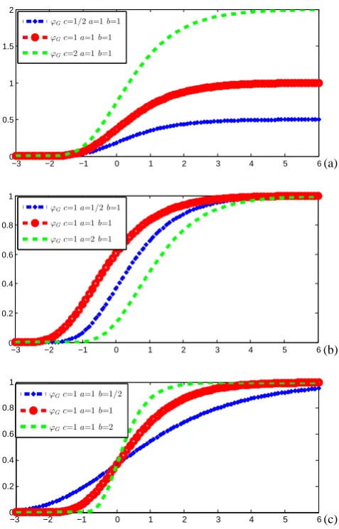
The Gompertz function is usually employed as a distribu-tion in survival analysis. This funcdistribu-tion was originally formu-lated by Gompertz (1825) for modeling human mortality. A number of authors contributed to the studies of the charac-terization of this distribution (e.g., Chen, 1997; Wu and Lee, 1999). In the field of water resources, the Gompertz function was adopted by Ouarda et al. (1995) to estimate the flood damage in the residential sector. The functionϕGis

increas-ing, flexible and continuous (Zimmerman and N´u˜nez-Ant´on, 2001). The Gompertz distribution has different formulations one of which is given by

ϕG(x)=cexp

n

−a e−bxo a, b, c >0; x ∈R, (3) wherecis its upper limit,aandbare two coefficients which respectively allow to translate and change the spread of the curve. Figure 1 shows the effects of these coefficients on the form of ϕG. Note that this function starts at zero (starting

phase), then increases exponentially (growth phase) and fi-nally stabilizes by approaching the upper limitc(stationary phase) with 0≤ϕG(x)≤c. The inflection point of this

func-tion isln_ba,c_e.

−3 −2 −1 0 1 2 3 4 5 6 0

0.5 1 1.5 2

ϕGc=1/2a=1b=1

ϕGc=1a=1b=1

ϕGc=2a=1b=1

a)

(a)

−3 −2 −1 0 1 2 3 4 5 6 0

0.2 0.4 0.6 0.8 1

ϕGc=1a=1/2b=1

ϕGc=1a=1b=1

ϕGc=1a=2b=1

b)

(b)

−3 −2 −1 0 1 2 3 4 5 6 0

0.2 0.4 0.6 0.8 1

ϕGc=1a=1b=1/2

ϕGc=1a=1b=1

ϕGc=1a=1b=2

c) _(c)

Fig. 1. Illustration of Gompertz function: (a)cvaries with fixeda

andb, (b)avaries with fixedbandcand (c)bvaries with fixeda

andc.

2.2.2 Logistic function

Verhuls (1838) proposed this function to study population growth. It is given by

ϕlogistic(x)=

c

1+a e−bx a, b, c >0; x ∈R, (4)

where the coefficientsc,aandbplay the same role as inϕG.

This function has similar properties to those of ϕG

(increasing, flexible, continuous and with three phases). However, ϕlogistic is symmetric around its inflection point

lna b ,

c

2

2.2.3 Linear function

It is a simple function, linear over three pieces corresponding to the three previous phases. Explicitly it is given by

ϕLinear(x)=

  

0 ifx ≤d1

x−d1

d2−d1 ifd1≤ x ≤d2, d2> d1 >0

1 ifx ≥d2

. (5)

This function is considered as a weight function in the study of Chebana and Ouarda (2008).

2.2.4 Indicator function

This function is given by ϕI(x)=

1 ifx ∈A

0 ifx /∈A, (6)

whereAis a subset in R (set of real numbers), such as an interval. The subsetArepresents the neighborhood or the re-gion in the classical RFA approaches. The weight is equal to 1 if the site is included in the region, otherwise, it is 0.

In the case where the setAis the interval [Cα,p, 1] with

Cα,p=₁₊1_χ2

α,p

andχ_α,p2 is the (1−α) quantile associated to the chi-squared distribution withp degrees of freedom, the DBRFA reduces to the traditional CCA approach (e.g., Bates et al., 1998). The corresponding weight function is denoted byϕCCA.

IfA= [0, 1], i.e.,α= 0, then the DBRFA represents the uni-form approach, which includes all available sites with similar importance. The corresponding weight function is denoted byϕU.

2.3 Weighted least squares estimation

In the RFA framework, the MR model is generally used to describe the relationship between the hydrological variables and the physiographical and climatic variables of the sites of a given region. This model has the advantage to be simple, fast, and not requiring the same distribution for hydrological data at each site within the region (Ouarda et al., 2001).

Let QT be the quantile corresponding to the return pe-riodT. It is often assumed that the relationship between QT, as the hydrological variable, and the physio-meteorological variables and basin characteristicsA1,A2, . . . ,Artakes the

form of a power function (Girard et al., 2004):

QT=β0Aβ₁1Aβ₂2 . . . Aβrr e, (7)

whereeis the model error.

Let s be the number of quantiles QT corresponding to s return periods and N be the total number of sites in the region. A matrix of hydrological variables Y = (QT1,

QT2, . . . ,QTs) of dimensionN×sis then constructed. With

a log-transformation in Eq. (7) we obtain the multivariate log-linear model in the following form:

log Y=(log X) β+ε, (8)

where log X = (1, logA1, logA2, . . . , logAr) is the

N×(r+1) matrix formed by (r) physio-meteorological variables series, β is the (r+1)×s matrix of parameters andε= (ε1, . . . ,εs)is the N×s matrix that represents the model error (residual) with null mean vectors and variance-covariance matrix0:

E(ε)=(0, . . . ,0)and Var(ε)=0=

  

Var ε1

. . .Cov ε1_{, ε}s ..

. . ...

Cov εs, ε1. . .Var(εs)   . (9)

The parameter matrixβ can be estimated, using the WLS estimation, by

ˆ βw =

arg min

β

(log Y−log Xβ)0 (log Y−log Xβ) =((log X)0log X)−1(log X)0log Y, (10) where= diag (w1, . . . ,wN) is the diagonal matrix with

di-agonal elementswiwherewi is the weight for the sitei. The

matrix0is estimated by

ˆ 0w=

log Y−log X_βˆ

w

0

log Y−log X_βˆ

w

N −r−1 . (11)

Note that the log-transformation induces generally a bias in the estimation of QT (Girard et al., 2004).

3 Methodology

This section describes a general procedure for optimizing the DBRFA approach and treats special cases where this procedure is applied using the weight functions defined in Sect. 2.2.

3.1 General procedure

In order to find the optimal weight functionϕOptimal in the

DBRFA approach, the procedure is composed of three main steps. They are summarized as follows:

1. For a given class of weight functions ϕ and a set of gauged sites (region), use a jackknife procedure to as-sess the regional flood quantile estimators (Eq. 8) for the sites of the region using the DBRFA approach. These estimators depend on the weight functionϕ through its coefficients.

3. Using an optimization algorithm, optimize the criterion (objective function) calculated in step (ii). The parame-ters of the optimization problem are the coefficients of the weight function. The outputs of this step areϕOptimal

and the value of the selected criterion.

3.2 Description of the procedure

In the first step of the procedure, we use a jackknife resam-pling procedure to assess the regional flood quantile esti-mators for the sites of the region. This jackknife procedure consists in considering each site l (l= 1, . . . , N) in the re-gion as an ungauged one by removing it temporarily from the region (i.e., we assume that the hydrological variable Ylof sitel is unknown and the physio-meteorological

vari-ableXl is known since it can be easily estimated from

ex-isting physiographic maps and climatic data). Then we cal-culate the regional estimatorYˆl

ϕ of sitel by the iterative

WLS regression, using theN−1 remaining sites, which is related to the given weight function ϕ. The parameters of the starting estimator (initial point) of DBRFA, denoted by

ˆ

β1,l and 0ˆ1,l, are calculated by assuming that X = X<−l>, Y = Y<−l>and= IN−1in Eqs. (10) and (11), whereX<−l>

represents the matrix of physio-meteorological variables ex-cluding sitel, Y<−l>is the matrix of hydrological variables excluding site l and IN−1 is the identity matrix of

dimen-sion (N−1)×(N−1). The starting estimator(Yˆ1,l)ϕ is

ob-tained by replacing β withβˆ1,l in Eq. (8). Then for each

depth iterationk,k= 2, 3, . . . ,kiter, we calculate the

Maha-lanobis depth (Eq. 2) of the gauged sitei,i= 1, . . . , N−1, with respect to the ungauged sitel denoted by Dk,(i,l)_ϕ=

MHD₍₀ˆ

k−1,l)ϕ

log Yi;

logYkˆ −1,l

ϕ

. The number of iter-ationskiter is fixed to ensure the convergence of the depth

function (generallykiter= 25 is appropriate). The weight

ma-trix at iterationkis defined by applying the functionϕto the depth calculated at this iteration. The parameters of the MR model at thek-th iteration are estimated by

ˆ

βk,l

ϕ =

log X<−l>0

k,l_ϕ

log X<−l>−1

log X<−l>0

k,l_ϕlog Y<−l>,(12)

ˆ

0k,l

ϕ =

log Y<−l>_{− log X}<−l>

ˆ

βk,l

ϕ 0

log Y<−l>_{− log X}<−l>

ˆ

βk,l

ϕ

(N−1)−r−1 ,(13)

where k,l

ϕis aN−1 diagonal matrix with elements:

ϕh Dk,(1,l)_ϕ

i

, . . . , ϕh Dk,(N−1,l)_ϕ

i

. (14)

Note that all these parameters depend onϕ. Then, the re-gional quantile estimator for the sitelin this iteration is

ˆ

Yk,l

ϕ

=exp

(log Xl)

ˆ βk,l

ϕ

. (15)

In the second step of the procedure, we use the regional es-timators at the last iteration since their associated estimation

errors are the minimum possible by construction. Conse-quently, in order to simplify the notations in the rest of this paper, we denote

ˆ

Y1

ϕ

=Yˆkiter,1

ϕ, . . . ,

ˆ

Yl

ϕ

=Yˆkiter,l

ϕ,

. . . , YˆN

ϕ

=Yˆkiter,N

ϕ.

After calculating(Yˆl)ϕ,l= 1, . . . ,N in step (i), we

con-sider and evaluate one or several performance criteria in step (ii). The considered criteria are employed as objective functions in the optimization step (iii).

The relative bias (RB) and the relative root mean square error (RRMSE) are widely used in hydrology, particularly in RFA, as criteria to evaluate model performances. These two criteria are defined using an element-by-element division by

RBϕ =100×

1 N

N

X

l=   

Yl−

ˆ

Yl

ϕ

Yl

 

, (16)

RRMSEϕ =100×

v u u u u t

1

N −1

N

X

l=1

  

Yl−

ˆ

Yl

ϕ

Yl

  

2

, (17)

where Yl is the local quantile estimation for the l-th site,

(Yˆl)ϕis the regional estimation by DBRFA approach

accord-ing toϕand excluding sitel, andN is the number of sites in the region. The RBϕ measures the tendency of quantile

esti-mates to be uniformly too high or too low across the whole region and the RRMSEϕ measures the overall deviation of

estimated quantiles from true quantiles (Hosking and Wallis, 1997). Note that other criteria can also be considered such as the Nash criterion (NASH) and the coefficient of determi-nation (R2). In the hydrological framework, the previously defined criteria are used as key performance indicators (KPI) to compare different RFA approaches (e.g., Ga´al et al., 2008). Finally in step (iii), we apply an optimization algorithm on the selected and evaluated criterion in step (ii). The al-gorithms to be considered are indicated in the introduction section. The formulation of the criteria to be optimized, gen-erally complex and non-explicit, suggests the use of zero-order algorithms. The application of these algorithms allows us to find the optimal function ϕOptimal with respect to

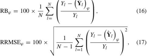
se-lected criteria. An overview diagram summarizing the opti-mization procedure of the DBRFA approach is illustrated in Fig. 2.

The procedure described above aims to calculateϕOptimal

according to the desired criterion. In order to estimate the quantileYuof an ungauged siteuusing the optimal DBRFA

 

 

N s

N r

Y Y

X X



     

 

Select: kiter, class ofφ, criterion and optimization method

Initialization site l=1

Exclude site l temporarily









1

1 1 l

N s

l N r

Y Y

X X

   

      

  

  

E

stim

at

e

Yl

u

si

n

g ite

rat

ive D

B

R

F

A

ap

p

roac

h

Compute ˆ_1,land ˆ_1,l Eq. (10) and (11) using  _1,l I_N₁

Starting estimator

 





k=2

Compute _{ }





1 - ,1 1 1

, , k log , logi ˆk l ; , ..,

k i l

D MHD_ Y Y i N

Update  using φ and D:

 













, , , , ..., , ,

k l diag  Dk l  Dk Nl  

Re-estimate ˆk l,and ˆk l,using k l,

Update ˆ_, k l

Y using the ˆk l, and ˆk l,

iter kk

  



lN

Compute the selected criterion as parametric function Start

Yes

Yes No

No

Jac

k

kni

fe

p

roc

ed

u

re

k

=

k

+1

l

=

l

+1

Output:_Optimal and the corresponding criteria

End

Optimize the criterion using the selected optimization method Input data

Hydrological

Physio-meteorological

Fig. 2. An overview diagram summarizing the optimization procedure of the DBRFA approach.

Based on the optimization procedure of the DBRFA ap-proach described previously, the parameters of the optimiza-tion problem are the coefficients of the weight funcoptimiza-tion. Con-sequently, reducing the number of coefficients inϕcan make the algorithm more efficient and less expensive in terms of

the valuec= 1 is fixed. In this case, the problem is reduced to find the couple (aˆN, bˆN) that optimizes one of the

pre-selected criteria, such as Eqs. (16) and (17).

Moreover, in the classes ϕ=ϕG or ϕ=ϕlogistic, the

opti-mization problem is applied in semi-bounded domain (i.e., a >0 andb >0) and without other constraints (linear or non-linear). In this case, the Nelder–Mead algorithm can also be applied as well as the pattern search one (Luersen and Le Riche, 2004).

On the other hand, in the case whereϕ=ϕLineair (Eq. 5),

the inequality constraintd2> d1>0 is imposed. Therefore,

the Nelder–Mead algorithm cannot be considered.

Theoretically and generally, the two optimization algo-rithms used in this paper (i.e., the Nelder–Mead and the pattern search algorithms) converge to a local minimum (or maximum) according to the initial point. To overcome this problem and make the algorithm more efficient, two solu-tions are proposed in the literature: (a) for each objective function, use several starting points and calculate the opti-mum for each of these points; the optiopti-mum of the function will be the best value of these local optima (Bortolot and Wynne, 2005); or (b) use a single starting point and each time the algorithm converges, the optimization algorithm restarts again using the local optimum as a new starting point. This procedure is repeated until no improvement in the optimal value of the objective function is obtained (Press et al., 2002).

4 Data sets for case studies

In this section we present the data sets on which the DBRFA approach will be applied in the following section. These data come from three geographical regions located in the states of Arkansas and Texas (USA) and in the southern part of the province of Quebec (Canada). The first region is lo-cated between 45 and 55◦N in the southern part of Que-bec, Canada. The data set of this region is composed of 151 stations, each station has a flood record of more than 15 yr. The conditions of application of frequency analysis (i.e., homogeneity, stationary and independence) are tested on the historical data of these stations in several studies (Chokmani and Ouarda, 2004; Ouarda and Shu, 2009; Shu and Ouarda, 2008). Three types of variables are considered: physiographical, meteorological and hydrological. The se-lected variables for the regional modeling are also used in Chokmani and Ouarda (2004). The selected physiographical variables are the basin area (AREA) in km2, the mean basin slope (MBS) in % and the fraction of the basin area covered with lakes (FAL) in %. The meteorological variables are the annual mean total precipitation (AMP) in mm and the annual mean degree days over 0◦C (AMD) in degree-day. The se-lected hydrological variables are represented by at-site spe-cific flood quantiles (QST) in m3km−2s, corresponding to return periodsT= 10 and 100 yr.

The two other considered regions correspond to a database of the United States Geological Survey (USGS). This database, called Hydro-Climatic Data Network (HCDN), consists of observations of daily discharges from 1659 sites across the United States and its Territories (Slack et al., 1993). The sites included in this database contain at least 20 yr of observations. As part of the HCDN project, the United States is divided into 21 large hydrological regions.

In this study, the data of the states of Arkansas and Texas (USA) are used for comparison purposes. The applicability conditions of frequency analysis as well as the variables to consider are justified in the study of Jennings et al. (1994). The physiographical and climatological characteristics are the area of drainage basin (AREA) in km2, the slope of main channel (SC) in m km−1, the annual mean precipitation (AMP) in cm, the mean elevation of drainage basin (MED) in m and the length of main channel (LC) in km. The se-lected hydrological variables in these two regions are the at-site flood quantiles (QT), in m3s−1corresponding to the re-turn periodsT = 10 and 50 yr.

The data set of the state of Arkansas is composed of 204 sites. These data and the at-site frequency analysis are published in the study of Hodge and Tasker (1995). Tasker et al. (1996) used these data to estimate the flood quantiles corresponding to the 50 yr return period by the region of in-fluence method (Burn, 1990b).

The Texas database is composed of 90 sites but due to the lack of some explanatory variables at several sites, modeling was performed with only 69 stations. The data set used in this region is the same used by Tasker and Slade (1994).

5 Results

The results obtained from the CCA-based approach are first presented and then compared to those obtained by the opti-mized DBRFA approach.

The variations of the two performance criteria RB and RRMSE, obtained by the CCA approach, as a function of the coefficientα(neighborhood coefficient) for the three regions are presented in Fig. 3. The complete variation range ofαis the interval [0, 1]. However, in this application, the range is [0, 0.30] for Quebec and Arkansas regions and [0, 0.17] for the Texas region. These upper bounds ofαare fixed to ensure that all neighborhoods of the sites contain sufficient stations to allow the estimation by the MR model. Note that it is ap-propriate to have at least three times more stations than the number of parameters in the MR model (Hach´e et al., 2002). Figure 3 indicates that, for a given region, the same value of αoptimizes the two criteria for the various return periods, even though this is not a general result (Ouarda et al., 2001). The optimalαvalues are 0.25, 0.01 and 0.05 respectively for Quebec, Arkansas and Texas.

The coefficients λ1 and λ2 correspond respectively to

0 0.1 0.2 0.3 −11 −10 −9 −8 −7 −6 −5 α %RB

0 0.1 0.2 0.3 44 46 48 50 52 54 56 58 60 62 64 α %RRMSE RB QS10 RB QS100 RRMSE QS10 RRMSE QS100 a) (a)

0 0.1 0.2 0.3 −22 −20 −18 −16 −14 −12 −10 −8 −6 α %RB RB Q10 RB Q50

0 0.1 0.2 0.3 50 60 70 80 90 100 α %RRMSE RRMSE Q10 RRMSE Q50 b) _(b)

0 0.05 0.1 0.15 −25 −20 −15 −10 −5 0 α %RB RB Q10 RB Q50

0 0.05 0.1 0.15 40 60 80 100 120 140 160 180 α %RRMSE RRMSE Q10 RRMSE Q50 c) (c)

Fig. 3. Optimal value of the neighborhood coefficientαfor the CCA

approach for (a) southern Quebec, (b) Arkansas and (c) Texas. The first column illustrates the RB and the second column illustrates the RRMSE.

canonical variables. Their values for Arkansas (λ1= 0.973,

λ2= 0.470) and Texas (λ1= 0.923,λ2= 0.402) are larger than

those of Quebec (λ1= 0.853,λ2= 0.281). This corresponds

to a large optimal value ofα for the latter region. Indeed, the higher the canonical correlation, the smaller the size of the ellipse defining the homogeneous neighborhood (Ouarda et al., 2001). The value of α should be small enough so that the neighborhood contains an appropriate number of sta-tions to perform the estimation in the MR model, and large enough to ensure an adequate degree of homogeneity within the neighborhood.

Figure 4 shows the projection sites of the three re-gions in the two canonical spaces (V1, W1) and (V2, W2)

−4 −2 0 2 4 −2 −1 0 1 2 3 4 1 2 3 4 5 6 7 8 9 10 11 12 13 14 15 16 17 18 19 20 21 22 23 24 25 26 27 28 29 30 31 32 3334 35 36 37 38 39 40 41 42 43 44 45 46 47 48 49 50 51 52 53 54 55 56 57 58 59 60 61 ₆₂ 63 64 65 66 67 68 69 70 71 72 73 74 75 76 77 78 79 80 81 82 83 84 85 86 87 8889 90 9192 93 94 95 96 97 98 99 100 101 102 103 104105 106 107 108 109 110 111 112 113 114 115 116 117 118 119 120 121 122 123 124 125 126 127 128 129 130 131 132 133 134 135 136 137 138 139 140 141142 143 144 145 146147 148 149 150

V2 (λ₂ = 0.28115)

W2 (

λ2

= 0.28115)

−2 −1 0 1 2 3 −2 −1 0 1 2 3 1 2 3 4 5 6 7 8 9 10 11 12 13 14 15 16 17 18 19 20 21 22 23 24 25 26 27 28 29 30 31 32 33 34 35 36 37 38 39 ₄₀ 41 42 4344 45 46 47 48 49 50 51 52 53 54 55 56 57 58 59 60 61 62 63 64 65 66 67 68 69 70 71 7273 74 75 7677 7879 80 81 82 83 84 85 86 87 88 89

909192

93 94

95 96

97 9899100

101 102 103 104 105106 107108 109 110 111 112 113114 115116 117 118 119 120 121 122 123 124 125 126 127 128 129 130 131 132 133 134 135 136 137 138 139 140 141142 143 144 145 146 147 148 149150

V1 (λ₁ = 0.85395)

W1 ( λ1 = 0.85395) Coefficient of determination 0.73 a) (a) (b)

−2 0 2 −3 −2 −1 0 1 2 3 1 2 3 4 5 6 7 8 9 10 11 12 13 14 15 16 17 18 19 20 21 22 23 24 25 26 27 28 29 30 31 32 33 3435 36 37 38 39 40 41 42 43 44 45 46 47 48 49 50 51 52 53 54 55 56 57 58 59 60 61 62 63 6465 66 67 68

V1 (λ₁ = 0.92369)

W1 (

λ1

= 0.92369)

−4 −2 0 2 4 −2 −1.5 −1 −0.5 0 0.5 1 1.5 2 2.5 1 2 3 4 5 6 7 8 9 10 11 12 13 14 15 16 17 18 19 20 21 22 23 24 25 26 27 28 29 30 31 32 33 34 35 36 37 38 39 40 41 42 43 44 45 46 4748 49 50 51 52 53 54 55 56 57 58 59 60 61 62 63 64 65 66 67 68

V2 (λ₂ = 0.40244)

W2 ( λ2 = 0.40244) Coefficient of determination 0.85 c) (c)

Fig. 4. Scatterplot of sites in the canonical spaces (V1, W1) and (V2, W2) for (a) southern Quebec, (b) Arkansas and (c) Texas. The first column illustrates the canonical (V1, W1) space and the second column illustrates the (V2, W2) space.

corresponding respectively toλ1andλ2. This figure shows

and W1 for each region, it is seen that the linearity assump-tion is more respected in Arkansas and Texas than in Quebec (R_Arkansas2 = 0.94,R2_Texas= 0.85 andR2_Quebec= 0.73).

The previous results show that the values ofλ1,λ2,αand

R2can be used as indicators of the quality of the homogene-ity in a given region. In this application, the lower values of λ1,λ2 andR2 as well as the higher value ofαfor Quebec

compared to the values of the other two regions indicate that the Quebec region is less homogeneous than the two others. This conclusion needs to be verified by other criteria or sta-tistical tests.

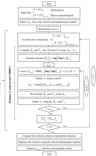
The DBRFA approach is applied by using the Mahalanobis depth function (Eq. 2). The optimal weight functions, from each one of the three considered families, are obtained on the basis of the indicated optimization algorithms (i.e.,ϕG and

ϕlogisticusing Nelder–Mead andϕLinearusing pattern search).

They are presented in Fig. 5. The corresponding results are summarized in Table 1. The optimization is made with re-spect to the RB and RRMSE criteria. Note that, for a given region, the regional flood quantile estimation is more accu-rate for small return periods. This result is valid for local as well as regional frequency analysis approaches (Hosking and Wallis, 1997). In addition, Table 1 shows that the worst estimates are obtained using the uniform approach (weight functionϕU). This justifies the usefulness of considering the

regional approaches. Note that for all regions, DBRFA with ϕOptimalleads to more accurate estimates in terms of RB and

RRMSE than those obtained using the CCA approach with optimalα. These results show also that the optimal coeffi-cients of a given weight function depend on the chosen cri-terion (objective function). Finally, for the southern Quebec region, the results of Chebana and Ouarda (2008) are very close to those in the present paper (Table 1). The reason for this closeness is that the above authors forced the DBRFA approach to provide good results by trying several different combinations of values ofϕcoefficients (i.e., iteration loop of coefficients). Consequently, their trials took a long time and did not ensure the optimality of the approach, which is not the case for the present study.

According to Fig. 5, the form of optimal weight function depends on the considered region. For instance, the steep S curve (with long upper extremity) of the two regions, Arkansas and Texas, depicts a large number of gauged sites similar to the target one; however, the high S curve (with short upper extremity) of Quebec shows a small number of gauged sites similar to the target one. This result supports the previously mentioned conclusion about the homogeneity level for these regions.

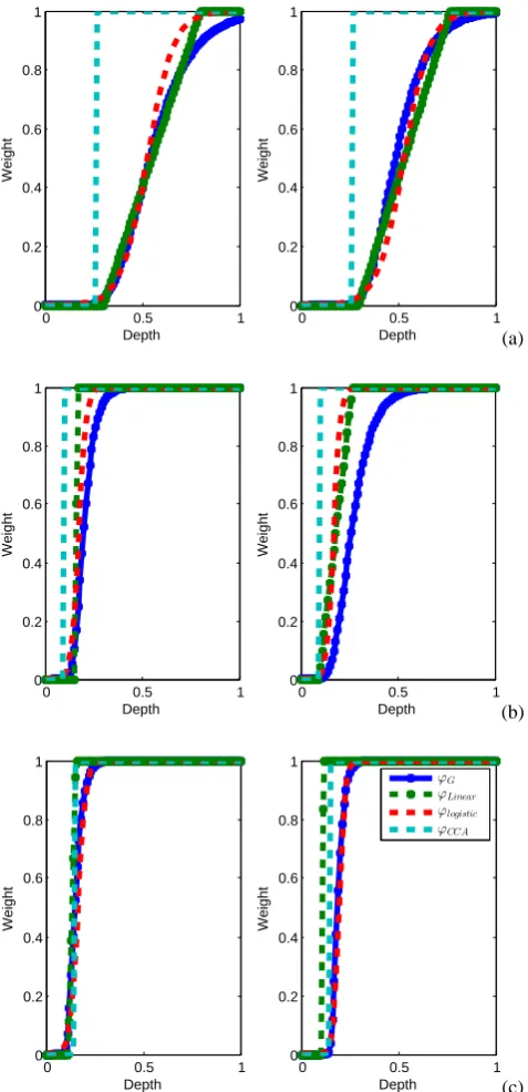
In order to visualize the influence of gauged sites on the regional estimation of a target site in the DBRFA and CCA approaches, assume that Texas site number 25 is a target site and has to be estimated using the remaining 68 gauged sites. Figure 6 illustrates the weights allocated to each gauged site in the canonical hydrological space (W1, W2) instead of the geographical space. The estimate is made with the optimal

0 0.5 1

0 0.2 0.4 0.6 0.8 1

Depth

Weight

0 0.5 1

0 0.2 0.4 0.6 0.8 1

Depth

Weight

a)

(a)

0 0.5 1

0 0.2 0.4 0.6 0.8 1

Depth

Weight

0 0.5 1

0 0.2 0.4 0.6 0.8 1

Depth

Weight

b)

(b)

0 0.5 1

0 0.2 0.4 0.6 0.8 1

Depth

Weight

0 0.5 1

0 0.2 0.4 0.6 0.8 1

Depth

Weight

ϕG ϕLinear ϕlogistic ϕCCA

c)

(c)

Fig. 5. Optimal weight functions for (a) southern Quebec, (b) Arkansas and (c) Texas. The first column illustrates the weight function’s optimal with respect to RRMSE and the second column illustrates the weight function’s optimal with respect to RB.

αfor the CCA approach and the optimalϕGfor the DBRFA

(a)

(b)

Fig. 6. Weight allocated to each gauged site to estimate the target-site number 25 in the Texas region in the canonical hydrological space (W1, W2) using (a) CCA with optimalαand (b) the DBRFA approach with optimalϕG.

weight function (Eq. 6) takes only two values: 1 within the neighborhood of the target site or 0 otherwise (Fig. 6a).

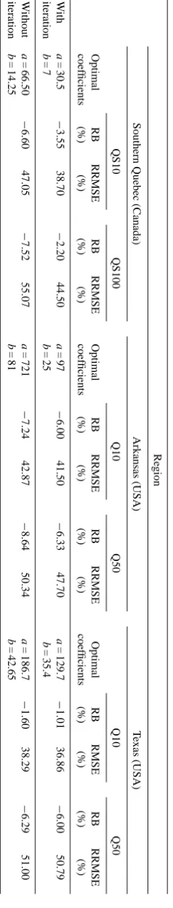
To study the impact of depth iterations on the perfor-mance of the DBFRA method, this approach is applied to the three regions but without iterations on the Mahalanobis depth (i.e., kiter= 2 in step (i) in the DBRFA optimization

procedure). The outputs of this application, withϕ=ϕG and

ζ(.) = RRMSE, are shown in Table 2. These results indicate that the optimal weight function changes depending on the case (with or without iterations) but keeps theS shape (for space limitation, the associated figure is not presented). In addition, using the iterations, we observe an improvement in the performance of the DBRFA method. This improvement varies from one region to another, where it is more signifi-cant in Quebec than in Texas and Arkansas (Table 2). This is another result indicating a difference between Quebec and the two other regions. Note that similar results are found for other families of weight functions and for different op-timization criteria. In conclusion, the depth iterative step in the DBRFA before weight optimization is important.

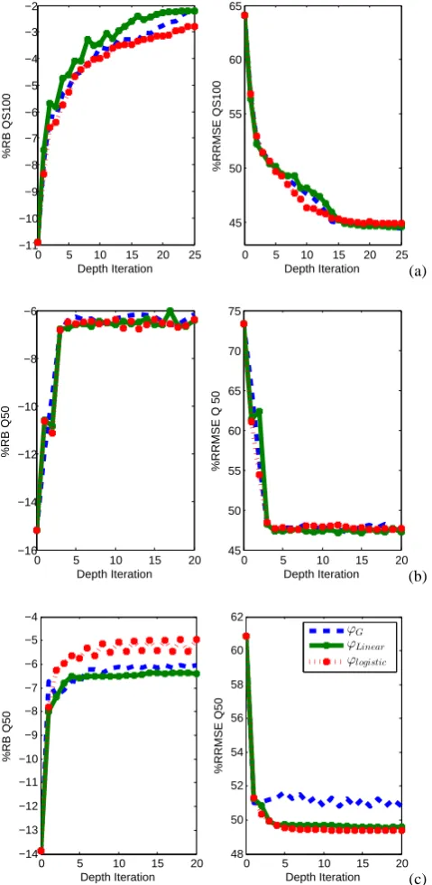
In order to examine the convergence speed in terms of the performance criteria, we present the variations of these crite-ria as a function of depth iteration for different weight func-tions (Fig. 7). The employed coefficient values of the weight

0 5 10 15 20 25 −11

−10 −9 −8 −7 −6 −5 −4 −3 −2

Depth Iteration

%RB QS100

0 5 10 15 20 25 45

50 55 60 65

Depth Iteration

%RRMSE QS100

a)

(a)

0 5 10 15 20 −16

−14 −12 −10 −8 −6

Depth Iteration

%RB Q50

0 5 10 15 20 45

50 55 60 65 70 75

Depth Iteration

%RRMSE Q 50

b)

(b)

0 5 10 15 20 −14

−13 −12 −11 −10 −9 −8 −7 −6 −5 −4

Depth Iteration

%RB Q50

0 5 10 15 20 48

50 52 54 56 58 60 62

Depth Iteration

%RRMSE Q50

ϕG ϕLinear ϕlogistic

c) _(c)

Fig. 7. Variation of criteria (RB and RRMSE) as a function of the depth iteration number for the estimation of (a) QS100 – southern Quebec, (b) Q50 – Arkansas and (c) Q50 – Texas.

functions are those minimizing the RRMSE (Table 1). We observe a rapid convergence (5 iterations) to the RRMSE val-ues in Table 1 for Arkansas and Texas (Fig. 7b, c), whereas, for Quebec (Fig. 7a) it requires more than 20 iterations to converge to the results in Table 1. These results could be again due to the level of homogeneity in the region.

T

able

2.

Results

of

the

DBRF

A

approach

with

and

without

depth

iterations

using

ζ

(.)

=

R

RMSE

and

ϕ

=

ϕ

G

.

Re

gion

Southern

Quebec

(Canada)

Arkansas

(USA)

T

exas

(USA)

QS10

QS100

Q10

Q50

Q10

Q50

Optimal

RB

RRMSE

RB

RRMSE

Optimal

RB

RRMSE

RB

RRMSE

Optimal

RB

RMS

E

RB

RRMSE

coef

ficients

(%)

(%)

(%)

(%)

coef

ficients

(%)

(%)

(%)

(%)

coef

fi

cients

(%

)

(%)

(%)

(%)

W

ith

a

=

30.5

−

3.55

38.70

−

2.20

44.50

a

=

97

−

6.00

41

.50

−

6.33

47

.70

a

=

129.7

−

1.01

36.86

−

6.00

5

0.79

iteration

b

=

7

b

=

25

b

=

35.4

W

ithout

a

=

66.50

−

6.60

47.05

−

7.52

55.07

a

=

721

−

7.24

42

.87

−

8.64

50

.34

a

=

186.7

−

1.60

38.29

−

6.29

5

1.00

iteration

b

=

14.25

b

=

81

b

=

(a)

(b)

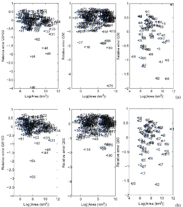
Fig. 8. Relative quantile errors using (a)ϕCCAand (b)ϕG. The first column illustrates the error of QS100 in southern Quebec, the second

column illustrates the errors of Q50 in Arkansas and the third column illustrates the errors of Q50 in Texas.

illustrates these errors with respect to the logarithm of basin area. The weight functions used are those optimizing the RRMSE. It is generally observed that the DBRFA relative errors are lower than those obtained with the CCA approach. We also observe large negative errors for some sites, such as number 64 and 66 in southern Quebec, 180 and 175 in Arkansas and 62 and 69 in Texas.

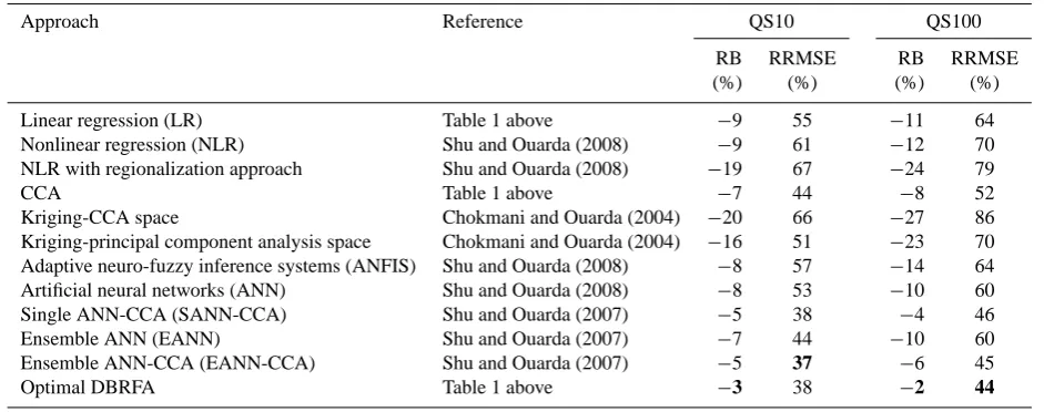
In this paper, the optimal DBRFA approach is mainly com-pared with the basic formulation of one of the most popular RFA approaches, which is the CCA approach. However, dif-ferent variants of the latter are developed and are available in the literature, such as the ensemble artificial neural networks-CCA approach (EANN-networks-CCA) (Shu and Ouarda, 2007) and the kriging-CCA approach (Chokmani and Ouarda, 2004). In order to insure the optimality of the optimal DBRFA, it is of interest to expend the above comparison to those approaches.

Table 3. Quantile estimation result for Quebec with available approaches and their references.

Approach Reference QS10 QS100

RB RRMSE RB RRMSE

(%) (%) (%) (%)

Linear regression (LR) Table 1 above −9 55 −11 64

Nonlinear regression (NLR) Shu and Ouarda (2008) −9 61 −12 70

NLR with regionalization approach Shu and Ouarda (2008) −19 67 −24 79

CCA Table 1 above −7 44 −8 52

Kriging-CCA space Chokmani and Ouarda (2004) −20 66 −27 86

Kriging-principal component analysis space Chokmani and Ouarda (2004) −16 51 −23 70

Adaptive neuro-fuzzy inference systems (ANFIS) Shu and Ouarda (2008) −8 57 −14 64

Artificial neural networks (ANN) Shu and Ouarda (2008) −8 53 −10 60

Single ANN-CCA (SANN-CCA) Shu and Ouarda (2007) −5 38 −4 46

Ensemble ANN (EANN) Shu and Ouarda (2007) −7 44 −10 60

Ensemble ANN-CCA (EANN-CCA) Shu and Ouarda (2007) −5 37 −6 45

Optimal DBRFA Table 1 above −3 38 −2 44

Best results are in bold character.

6 Conclusions

In the present paper, a procedure is proposed to optimize the selection of a weight function in the DBRFA approach. This procedure automates the optimal choice of the weight func-tionϕwith respect to a given criterion. Therefore, aside from leading to optimal estimation results, it allows the DBRFA approach to be more practical and usable without the user’s subjective intervention. The user has only to select one or several objective performance criteria to obtain the model, the estimated performance and the weight functions for a specific region. One of the findings is that the optimal weight function can be seen as characterization of the associated region.

General and flexible families of weight function are con-sidered, as well as two optimization algorithms to find ϕOptimal. The used algorithms can handle cases with or

with-out constraints on the definition domain of the functionϕ. The obtained results, from three regions in North America, show the utility of considering the DBRFA method in terms of performance as well as the efficiency and flexibility of the proposed optimization procedure.

The study of the three regions shows an association be-tween the level of the homogeneity of the region, the form of the optimal weight function and the computation conver-gence speed. This result deserves to be developed in future work.

Acknowledgements. Financial support for this study was graciously provided by the Natural Sciences and Engineering Research Coun-cil (NSERC) of Canada and the Canada Research Chair Program. The authors are grateful to the Editor and the anonymous reviewers for their valuable comments and suggestions.

Edited by: F. Laio

References

B´ardossy, A. and Singh, S. K.: Robust estimation of hydrologi-cal model parameters, Hydrol. Earth Syst. Sci., 12, 1273–1283, doi:10.5194/hess-12-1273-2008, 2008.

Bates, B. C., Rahman, A., Mein, R. G., and Weinmann, P. E.: Cli-matic and physical factors that influence the homogeneity of re-gional floods in southeastern Australia, Water Resour. Res., 34, 3369–3381, 1998.

Bortolot, Z. J. and Wynne, R. H.: Estimating forest biomass using small footprint LiDAR data: An individual tree-based approach that incorporates training data, ISPRS J. Photogramm. Remote S., 59, 342–360, 2005.

Burn, D. H.: An appraisal of the “region of influence” approach to flood frequency analysis, Hydrolog. Sci. J./Journal des Sciences Hydrologiques, 35, 149–165, 1990a.

Burn, D. H.: Evaluation of regional flood frequency analysis with a region of influence approach, Water Resour. Res., 26, 2257– 2265, 1990b.

Chebana, F.: On the optimization of the weighted Bickel– Rosenblatt test, Stat. Probab. Lett., 68, 333–345, 2004.

Chebana, F. and Ouarda, T. B. M. J.: Depth and homogeneity in regional flood frequency analysis, Water Resour. Res., 44, W11422, doi:10.1029/2007WR006771, 2008.

Chebana, F. and Ouarda, T. B. M. J.: Depth-based multivariate de-scriptive statistics with hydrological applications, J. Geophys. Res.-Atmos., 116, D10120, doi:10.1029/2010JD015338, 2011a. Chebana, F. and Ouarda, T. B. M. J.: Multivariate extreme value identification using depth functions, Environmetrics, 22, 441– 455, 2011b.

Chen, Z.: Parameter estimation of the Gompertz population, Biometr. J., 39, 117–124, 1997.

Chokmani, K. and Ouarda, T. B. M. J.: Physiographical space-based kriging for regional flood frequency estimation at ungauged sites, Water Resour. Res., 40, 1–13, 2004.

De Michele, C. and Rosso, R.: A multi-level approach to flood frequency regionalisation, Hydrol. Earth Syst. Sci., 6, 185–194, doi:10.5194/hess-6-185-2002, 2002.

Dolan, E. D., Michael Lewis, R., and Torczon, V.: On The Local Convergence Of Pattern Search, SIAM J. Optim., 14, 567–583, 2003.

Ga´al, L., Kysel´y, J., and Szolgay, J.: Region-of-influence approach to a frequency analysis of heavy precipitation in Slovakia, Hy-drol. Earth Syst. Sci., 12, 825–839, doi:10.5194/hess-12-825-2008, 2008.

Girard, C., Ouarda, T. B. M. J., and Bob´ee, B.: Study of bias in the log-linear model for regional estimation, ´Etude du biais dans le mod`ele log-lin´eaire d’estimation r´egionale, Can. J. Civil Eng., 31, 361–368, 2004.

Gompertz, B.: On the nature of the function expressive of the law of human mortality, and on a new mode of determining the value of life contingencies, Philos. T. Roy. Soc. Lond., 115, 513–585, 1825.

GREHYS: Presentation and review of somemethods for regional flood frequency analysis, J. Hydrol., 186, 63–84, 1996a. Hach´e, M., Ouarda, T. B. M. J., Bruneau, P., and Bob´ee, B.:

Re-gional estimation by canonical correlation analysis: Hydrolog-ical variable analysis, Estimation r´egionale par la m´ethode de l’analyse canonique des corr´elations: Comparaison des types de variables hydrologiques, Can. J. Civil Eng., 29, 899–910, 2002. Haddad, K. and Rahman, A.: Regional flood frequency analysis

in eastern Australia: Bayesian GLS regression-based methods within fixed region and ROI framework – Quantile Regression vs. Parameter Regression Technique, J. Hydrol., 430–431, 142– 161, 2012.

Hereford, J.: Comparison of four parameter selection techniques, Proceedings of SoutheastCon 2001, 30 March–1 April 2001, Clemson, SC, 11–16, 2001.

Hodge, S. A. and Tasker, G. D.: Magnitude and Frequency of Floods in Arkansas, US Geological Survey Water-Resources Investi-gations Report, US Geological Survey, Denver, Colo., 277 pp., 1995.

Hooke, R. and Jeeves, T. A.: Direct search solution of numerical and statistical problems, J. Assoc. Comput. Mach., 8, 212–229, 1961.

Hosking, J. R. M. and Wallis, J. R.: Regional frequency analysis: an approach based on L-moments, Cambridge University Press, Cambridge, 1997.

Jennings, M. E., Thomas Jr., W. O., and Riggs, H. C.: Nationwide summary of U.S. geological survey regional regression equations for estimating magnitude and frequency of floods for ungaged sites, 1993, USGS Water-Resources Investigations Rep. 94-4002, Reston, Virginia, 1994.

Krauße, T. and Cullmann, J.: Towards a more representative parametrisation of hydrologic models via synthesizing the strengths of Particle Swarm Optimisation and Robust Pa-rameter Estimation, Hydrol. Earth Syst. Sci., 16, 603–629, doi:10.5194/hess-16-603-2012, 2012.

Krauße, T., Cullmann, J., Saile, P., and Schmitz, G. H.: Robust multi-objective calibration strategies – possibilities for improv-ing flood forecastimprov-ing, Hydrol. Earth Syst. Sci., 16, 3579–3606, doi:10.5194/hess-16-3579-2012, 2012.

Lewis, R. M. and Torczon, V.: Pattern search algorithms for bound constrained minimization, SIAM J. Optim., 9, 1082–1099, 1999.

Lewis, R. M. and Torczon, V.: A globally convergent augmented La-grangian pattern search algorithm for optimization with general constraints and simple bounds, SIAM J. Optim., 12, 1075–1089, 2002.

Liu, R. Y. and Singh, K.: A quality index based on data depth and multivariate rank tests, J. Am. Stat. Assoc., 88, 252–260, 1993. Luersen, M. A. and Le Riche, R.: Globalized nelder-mead method

for engineering optimization, Comput. Struct., 82, 2251–2260, 2004.

Madsen, H. and Rosbjerg, D.: Generalized least squares and em-pirical Bayes estimation in regional partial duration series index-flood modeling, Water Resour. Res., 33, 771–781, 1997. Mahalanobis, P. C.: On the generalized distance in statistics,

Cal-cutta Statist. Assoc. Bull., 14, p. 9, 1936.

McKinnon, K. I. M.: Convergence of the Nelder-Mead simplex method to a nonstationary point, SIAM J. Optim., 9, 148–158, 1999.

Nelder, J. A. and Mead, R.: A simplex method for function mini-mization, Comput. J., 7, 308–313, 1965.

Nguyen, V.-T.-V. and Pandey, G.: A new approach to regional es-timation of floods in Quebec, in: Proceedings of the 49th An-nual Conference of the CWRA, Delisle, edited by: Bouchard, M. A., 26–28 June 1996, Collection Environnement de l’U: de Montr´eal, Quebec City, 587–596, 1996.

Ouarda, T. B. M. J. and Shu, C.: Regional low-flow frequency anal-ysis using single and ensemble artificial neural networks, Water Resour. Res., 45, W11428, doi:10.1029/2008WR007196, 2009. Ouarda, T. B. M. J., El-Jabi, N., and Ashkar, F.: Flood damage

es-timation in the residential sector. Water Resources and Environ-mental Hazards: Emphasis on Hydrologic and Cultural insight in the Pacific Rim, AWRA Technical Publication series 1995, AWRA, 73–82, 1995.

Ouarda, T. B. M. J., Hache, M., Bruneau, P., and Bobee, B.: Re-gional flood peak and volume estimation in northern Canadian basin, J. Cold Reg. Eng., 14, 176–191, 2000.

Ouarda, T. B. M. J., Girard, C., Cavadias, G. S., and Bob´ee, B.: Regional flood frequency estimation with canonical correlation analysis, J. Hydrol., 254, 157–173, 2001.

Ouarda, T. B. M. J., Bˆa, K. M., Diaz-Delgado, C., Cˆarsteanu, A., Chokmani, K., Gingras, H., Quentin, E., Trujillo, E., and Bob´ee, B.: Intercomparison of regional flood frequency estimation meth-ods at ungauged sites for a Mexican case study, J. Hydrol., 348, 40–58, 2008.

Press, W. H., Flannery, B. P., Teukolsky, S. A., and Vetterling, W. T.: Numerical recipes in C: the art of scientific computing, 2nd Edn., Cambridge University Press, New York, 1002 pp.+xxviii, 2002. Rao, S. S.: Engineering Optimization-Theory and Practice,

3rd Edn., John Wiley & Sons, 621–622, 1996.

Rosenbrock, H. H.: An automatic method for finding the greatest or least value of a function, Comput. J., 3, 175–184, 1960. Shu, C. and Ouarda, T. B. M. J.: Flood frequency analysis at

un-gauged sites using artificial neural networks in canonical cor-relation analysis physiographic space, Water Resour. Res., 43, W07438, doi:10.1029/2006WR005142, 2007.

Slack, J. R., Lumb, A. M., and Landwehr, J. M.: Hydro-Climatic Data Network (HCDN): Streamflow data set, 1874–1988, Hydro-climatic Data Network (HCDN): A US Geological Survey Streamflow Data Set for the United States for the Study of Cli-mate Variations, 1874–1988, US Geological Survey, Reston, Vir-ginia, USA, 1993.

Tasker, G. D. and Slade, R. M.: An interactive regional regres-sion approach to estimating flood quantiles, Water Policy and Management: Solving the Problems, ASCE Proceedings of the 21st Annual Conference of the Water Resources Planning and Management Division, New York, 782–785, 1994.

Tasker, G. D., Hodge, S. A., and Barks, C. S.: Region of influence regression for estimating the 50-year flood at ungaged sites, J. Am. Water Resour. Assoc., 32, 163–170, 1996.

Torczon, V.: On the Convergence of Pattern Search Algorithms, SIAM J. Optim., 7, 1–25, 2000.

Tukey, J. W.: Mathematics and the picturing of data, Vol. 2, Pro-ceedings of the International Congress of Mathematicians, Van-couver, B.C., 1974, Canad. Math. Congress, Montreal, Quebec, 523–531, 1975.

Verhulst, P. F.: Notice sur la loi que la population pursuit dans son accroissement, Correspondance Math´ematique et Physique, 10, 113–121, 1838.

Wright, M. H.: Direct Search Methods: Once Scorned, Now Re-spectable, in: Numerical Analysis 1995, Papers from the Six-teenth Dundee Biennial Conference held at the University of Dundee, Dundee, 27–30 June 1995, edited by: Griffiths, D. F. and Watson, G. A., Longman, Harlow, London, 191–208, 1996. Wu, J. W. and Lee, W. C.: Characterization of the mixtures of

Gom-pertz distributions by conditional expectation of order statistics, Biometr. J., 41, 371–381, 1999.

Zimmerman, D. L. and N´u˜nez-Ant´on, V.: Parametric modelling of growth curve data: An overview, Test, 10, 1–73, 2001.