Water vapor mapping by fusing InSAR and GNSS remote sensing data and atmospheric simulations

doi:10.5194/hess-19-4747-2015

© Author(s) 2015. CC Attribution 3.0 License.

Water vapor mapping by fusing InSAR and GNSS remote sensing

data and atmospheric simulations

F. Alshawaf1,3, B. Fersch2, S. Hinz1, H. Kunstmann2, M. Mayer3, and F. J. Meyer4

1_{Institute of Photogrammetry and Remote Sensing, Karlsruhe Institute of Technology (KIT), 76131 Karlsruhe, Germany} 2_{Institute of Meteorology and Climate Research, Campus Alpin, KIT, 82467 Garmisch-Partenkirchen, Germany} 3_{Geodetic Institute, KIT, 76131 Karlsruhe, Germany}

4_{Geophysical Institute, University of Alaska Fairbanks, Fairbanks, AK 99775, USA} Correspondence to: F. Alshawaf (fadwa.alshawaf@kit.edu)

Received: 19 November 2014 – Published in Hydrol. Earth Syst. Sci. Discuss.: 12 January 2015 Revised: 27 October 2015 – Accepted: 16 November 2015 – Published: 3 December 2015

Abstract. Data fusion aims at integrating multiple data sources that can be redundant or complementary to produce complete, accurate information of the parameter of interest. In this work, data fusion of precipitable water vapor (PWV) estimated from remote sensing observations and data from the Weather Research and Forecasting (WRF) modeling sys-tem are applied to provide complete grids of PWV with high quality. Our goal is to correctly infer PWV at spatially con-tinuous, highly resolved grids from heterogeneous data sets. This is done by a geostatistical data fusion approach based on the method of fixed-rank kriging. The first data set contains absolute maps of atmospheric PWV produced by combin-ing observations from the Global Navigation Satellite Sys-tems (GNSS) and Interferometric Synthetic Aperture Radar (InSAR). These PWV maps have a high spatial density and a millimeter accuracy; however, the data are missing in re-gions of low coherence (e.g., forests and vegetated areas). The PWV maps simulated by the WRF model represent the second data set. The model maps are available for wide areas, but they have a coarse spatial resolution and a still limited ac-curacy. The PWV maps inferred by the data fusion at any spa-tial resolution show better qualities than those inferred from single data sets. In addition, by using the fixed-rank kriging method, the computational burden is significantly lower than that for ordinary kriging.

1 Introduction

the simulated parameters (Pichelli et al., 2010; Bennitt and Jupp, 2008). We want to comprehend whether the model sim-ulations of water vapor, in their current quality, can be used to even out the deficits of the measurement-based estimates, particularly in regions with no measurements. To achieve this purpose, a statistical data fusion approach is applied. The output water vapor maps can be used in tomographic ap-proaches to provide 3-D water vapor grids and to adjust the parameters of numerical atmospheric prediction models. The remainder of this section presents the recent related research on water vapor using remote sensing data and atmospheric models.

The amount of remote sensing data available for moni-toring the Earth and its atmosphere is growing in a rapid, continuous way. InSAR has proved its capability for detect-ing surface deformation, landslides, and tectonic movements (Massonnet et al., 1993; Zebker et al., 1994), and for deriv-ing digital elevation models (Zebker and Goldstein, 1986). The influence of water vapor in the observations can be re-duced by averaging a large number of interferograms (Zebker et al., 1997) or by time series analysis that indicates the sta-ble persistent scatterers (Ferretti et al., 2001; Hooper et al., 2007). Besides, InSAR has recently been used to derive the phase shift caused due to the propagation in the Earth’s at-mosphere from the interferograms or by time series analy-sis (Hanssen, 2001; Meyer et al., 2008; Pichelli et al., 2010; Alshawaf et al., 2012). Global Navigation Satellite Systems (GNSS), however, have been considered since the 1990s as an efficient microwave-based tool for atmospheric sounding (Bevis et al., 1992; Rocken et al., 1995). Since then, numer-ous methods have exploited the GNSS observations to pro-duce estimates of the integrated atmospheric water vapor and to generate water vapor maps (Luo et al., 2008; Jade and Vi-jayan, 2008; Karabati´c et al., 2011). InSAR and GNSS, sig-nals are affected in a similar way by the atmosphere (Onn and Zebker, 2006). Therefore, Alshawaf et al. (2015b) presented a new approach to deriving absolute, high-resolution maps of precipitable water vapor (PWV) by combining data from InSAR and GNSS. The SAR systems acquire the images at repeat cycles of multiples of days. Enivsat images, which are used in this work, are available in multiples of 35 days. The availability of the data over time can be increased by pro-cessing data from ascending and descending modes. In addi-tion, new SAR missions have shorter repeat cycles, 11 days for TerraSAR-X and 6 days for Sentinel-1. The InSAR-based PWV estimates cannot be used to observe the variability of water vapor over a short time, but they are important in dif-ferent aspects. This geodetic-based method produces maps of the PWV at a high spatial resolution without additional costs. These data can be exploited, first, to model the spatial varia-tions of atmospheric turbulent and non-turbulent effects. Sec-ond, they can be used to observe the variation of water con-tent over long time periods to detect, for example, unusual trends. Third, they can be used to adjust/readjust the initial and boundary conditions in atmospheric prediction models.

Atmospheric modeling systems are standard approaches to simulate 3-D distributions of the neutrospheric water va-por at various temva-poral and spatial samplings. Dynamic local area models (LAMs) are common tools for scaling down the coarse grids of global circulation models to meso-scale ap-plicability. Several studies employed the Weather Research and Forecasting modeling system (WRF, Skamarock and Klemp, 2008) to compare the LAM simulations of PWV with GNSS point estimates (Mateus et al., 2010; Bender et al., 2008; Cimini et al., 2012) and PWV maps from MERIS (MEdium Resolution Imaging Spectrometer) (Al-shawaf et al., 2012). These studies conclude that the medium-to long-scale (greater than 20 km) water vapor signals can be well predicted, whereas short-scale fluctuations are often hardly captured in a realistic way.

Despite manifold improvements over the last years, con-siderable uncertainties are still connected with the parameter-ization of physical processes in mesoscale-atmospheric mod-els and biases of the driving model (Prein et al., 2015). This, in addition to the configuration of the model domains, can significantly impact the simulation output (Gong et al., 2010) as well as the model intrinsic water balance (Awan et al., 2011; Fersch et al., 2012; Fersch and Kunstmann, 2014). Therefore, the setup of the local area model is crucial, and it has to be proper for the study region and the research ob-jectives.

Figure 1. Maps of the absolute atmospheric PWV derived by combining PSI and GNSS data and the corresponding map from MERIS. The

spatial correlation is 95 % and the rms value of the differences is 0.68 mm.

2 Atmospheric water vapor

Several observation systems are commonly used to contin-uously monitor the vertical and horizontal distributions of water vapor in the atmosphere. These devices are used ei-ther from the ground, such as radiosondes and ground-based water vapor radiometers, or from space, such as space-based water vapor radiometers and infrared sensors. In this work, we employ microwave remote sensing systems as well as nu-merical atmospheric models to provide accurate maps of the atmospheric water vapor at a high spatial resolution. 2.1 Water vapor from remote sensing data

Alshawaf et al. (2015b) presented a new approach to derive absolute, high-resolution maps of PWV by combining data from InSAR and GNSS. The data are collected in the region of Upper Rhine Graben in Germany and France over the pe-riod 2003–2008. Persistent scatterer InSAR (PSI) using the Stanford Method for Persistent Scatterers (StaMPS, Hooper et al., 2007) was applied to derive PWV maps from the In-SAR interferograms. These maps contain the water vapor signal of short-scale spatial variations, while the elevation-dependent and long wavelength water vapor components are eliminated when forming the interferograms or by phase fil-tering. Therefore, GNSS-based PWV estimates were used to reconstruct the missing components. The approach for com-bining InSAR and GNSS data is presented in detail in Al-shawaf et al. (2015a) and AlAl-shawaf et al. (2015b). Figure 1 shows a map of PWV derived by combining PSI and GNSS data and the corresponding map extracted from MERIS ob-servations. MERIS is a passive imaging spectrometer located on board the Envisat platform. It measures the solar radiation reflected from the Earth’s surface or clouds. The ratio of the radiance values measured at channels 14 and 15, located re-spectively at 885 and 900 nm, are used to determine the verti-cal PWV content in the neutrosphere (Fischer and Bennartz, 1997). MERIS provides maps of the PWV at a spatial

reso-lution of 260 m×290 m (full-resolution mode). Under cloud weather conditions MERIS measurements are highly under-estimated since the measured PWV represents only the water vapor existing between the sensor and cloud top; therefore, only five MERIS PWV images were available for this study. The PSI method produces information where stable per-sistent scatterers are identified, which requires a high coher-ence between the SAR images. In forests and vegetated ar-eas, the probability of identifying persistent scatterers is low; therefore, in these regions, only sparse points are found. The white areas within the left figure indicate regions of low co-herence and the corresponding data from MERIS are masked out. The spatial correlation between the maps is 95 % and the root mean square (rms) value of the differences is 0.68 mm. We can observe that the persistent scatterers are dense in the urban areas, while they almost disappear in the low coher-ence regions. Since PWV data are spatial, their covariance function is exploited by geostatistical techniques to reason-ably infer the PWV at regular grids. In order to improve the inferred PWV maps, especially in the areas where the PWV estimates are sparse, we apply data fusion of the remotely sensed PWV maps with maps produced by the WRF model.

2.2 Water vapor from regional atmospheric models

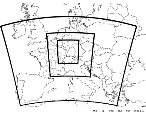
radia-Figure 2. WRF model set up with a parent domain of resolution

27 km×27 km and two nests of 9 km×9 km and 3 km×3 km, re-spectively.

tion was computed with the community atmospheric model (CAM) scheme (Collins et al., 2004). The processes in the planetary boundary layer were represented by the Yonsai University scheme (Hong et al., 2006). The surface layer was simulated with the Monin–Obukhov scheme, and the Noah land-surface model (Chen and Dudhia, 2001) was applied for the surface physics. Sub-grid convective processes were in-cluded with the Kain–Fritsch parametrization (Kain, 2004). The global dynamic boundary conditions were ingested from the European Center for Medium-Range Weather Forecasts (ECMWF) ERA-INTERIM reanalysis at a 6 h interval (Up-pala et al., 2008). In ERA-INTERIM, a broad range of dif-ferent data sources is assimilated. For the atmospheric mois-ture analysis, ground-based station observations, radiosonde profiles, and GPS radio occultation are exploited. Addition-ally, total column water vapor information from the Special Sensor Microwave/Imager (SSM/I) and the Advanced Mi-crowave Scanning Radiometer for the Earth Observing Sys-tem (AMSR-E) is assimilated (Dee et al., 2011). MERIS re-trievals of column water vapor are not ingested into ERA-INTERIM, and thus they depict an independent data set for our approach.

The WRF simulations cover the period between July 2004 and September 2005, such that the first 5 months were con-sidered as spin-up. The PWV content was determined at ev-ery output time step (10 min) by a vertical integration of all moisture fields from the land surface to the model top. Two output time slices were compared with the simultane-ous MERIS observations. The long-scale signal is modeled by a linear trend and subtracted from the maps; hence, neg-ative values are observed on the color bars. From the com-pared maps shown in Fig. 3, we observe that the spatial at-mospheric patterns are not always correctly resembled by the

model. On 27 June 2005 (09:51 UTC), WRF and MERIS PWV maps are strongly correlated with a coefficient of 0.8, whereas the analysis of 5 September 2005 (09:51 UTC) shows a lower spatial correlation (0.71). While the patterns east of the Upper Rhine valley are reasonably resembled, an unexpected discontinuity exists in the area around 7.7◦E, 48.7◦N.

At the lateral boundaries, WRF ingests the mixing ratio concentration from the global model. Thus, for the presented simulation, the global climate model lateral boundary condi-tions were applied to the first (outer) domain. Neither grid-ded nor spectral nudging was activated in order to conserve the model’s internal water balance. Hence the GCM bound-ary fluxes and the local area model physics solely determine the propagation of moisture through the respective domains. For the analysis of 27 June 2005, the atmospheric conditions were rather unexcited and varied slowly, resulting in a good agreement between MERIS and WRF data. On 5 September, a quickly moving frontal system with a strong west-to-east gradient and a notch in the atmospheric vapor over the Up-per Rhine Graben characterized the study region. It is not clearly distinguishable whether the structure and dynamics of the ERA-INTERIM boundaries or the WRF model con-figurations are responsible for the discontinuity in PWV.

3 Change of support problem

Spatial data, for which close observations correlate more than distant ones, can be collected at points or areal units. The former are called point-level data or simply point data and the latter are areal-level or block data (Gelfand et al., 2001). In geostatistics, this defines the spatial support of the data. When both data types are available, data fusion can be ap-plied to infer the underlying process at any level of support. The change of support problem is concerned with the infer-ence of the underlying process at point levels or block lev-els different from those at which the data are available. This also includes fusing data at different support levels. Based on the available input data and the desired output grid, there are four prediction possibilities: points to points, points to blocks, blocks to points, or blocks to blocks. These prediction possibilities may be collected under the umbrella of kriging (Cressie, 1993).

For block data that can be expressed as an average of point data as if it is collected within the block, such as rainfall, temperature, surface elevation, and atmospheric water vapor, the following model is appropriate:

Y (Bi)= 1 |Bi|

Z

Bi

Y (s)ds, (1)

Figure 3. Maps of PWV content as received from MERIS and WRF, where a linear trend is subtracted from each map. The upper data are

received on 27 June 2005 (09:51 UTC), the lower data on 5 September 2005 (09:51 UTC). Gaussian averaging is applied to scale the MERIS data at WRF resolution, 3 km×3 km. The spatial correlation coefficient between the upper maps is 0.8 and 0.71 for the lower maps.

data. The block-level covariance can then be related to the point-level covariance as follows:

C(Bi, Bj)=cov

  

1 |Bi|

Z

Bi

Y (u)du, 1

|Bj|

Z

Bj Y (v)dv

   (2)

= 1

|Bi||Bj|

Z

Bi

Z

Bj

C(u,v)dudv, (3)

whereC(Bi, Bj)is the block-to-block or block covariance function andC(u,v)is the point covariance function.

4 Spatial data fusion using kriging methods 4.1 Ordinary kriging

In geostatistics, a spatial process can be inferred over a con-tinuous spatial domain by exploiting the covariance func-tion as an important source of informafunc-tion. Predicfunc-tions are obtained based either on single or multiple sets. Kriging is a geostatistical interpolation technique that infers values at

+

Block B

+ +

+ +

+

+ +

+ +

+

+ +

+

+

+ +

+

+

+ Observed samples locations Regularly-spaced locations

+ +

Bi→Y(Bi)

s→Y(s)

Figure 4. Point and block data, such that for spatial data,Y (B_i) represents the average of the point data within the block.

ˆ

Y (s0)at the locations0is determined as follows: ˆ

Y (s0)=a0eZ, (4)

where the vector a contains the kriging weighting coeffi-cients and eZ is the centered data set (see Eq. 7). The best

linear unbiased estimator is found by solving the following constrained minimization problem:

min

a E

n

(Y (ˆ s)−Y (s))2

o

subject to

E{ ˆY (s)} =E{Y (s)}. (5) The constraint is added to guarantee that the estimator is unbiased with respect to the true processY (s). A semivar-iogram function that reflects the spatial correlations is re-quired to solve the minimization problem, which is deter-mined from the detrended data in Eq. A6.

The kriging method extends the spatial process using the following linear model:

Z(s)=T(s)·α+ν(s)

| {z }

Y(s)

+(s)

|{z}

noise

, (6)

where(s)is an independent error term, which is assumed to be a white noise process with a mean zero and varianceσ2. T(s)·α defines a deterministic linear trend, T has a size of

N×3 and each row has the following entries: [1 longitude(s) latitude(s)].Nis the number of observations andαis a vector of the least squares regression coefficient.ν(s)captures the spatial covariance structure of the process, and it is assumed to have a mean zero and generally a non-stationary covari-ance function. Before inferring the signal at a new location, it is required to center the data by estimating and subtracting the linear trend, i.e.,

e

Z=Z−Tαˆ with αˆ=(TT0)−1T0Z. (7)

The detrended signaleZ is used to determine the predictions

in Eq. (4) and the deterministic signal is calculated from

T(s0)αˆ. The sum of the two terms gives the total estimated value ofY (s0). In the next section, a similar strategy is fol-lowed to solve for the best unbiased estimator using two data sets as presented in Braverman et al. (2009).

4.2 Spatial statistical data fusion

Spatial statistical data fusion (SSDF) is a method that statisti-cally combines two data sets to optimally infer the quantity of interest and calculate the corresponding uncertainties at any predefined grid (Nguyen, 2009; Braverman et al., 2009). This method extends the kriging technique described above to find the optimal estimator using multiple data sets. Let the under-lying processY (s)to be estimated at the locationsfrom the data inZ1andZ2with the sizesN1andN2, respectively. The estimatorY (ˆ s)at the locationsis obtained from the two data sets as follows:

ˆ

Y (s)=a0₁eZ1+a02eZ2, (8)

wherea1anda2 are the fusion weighting coefficients, and

e

Z1andeZ2are detrended data sets ofZ1andZ2, respectively. Following Eq. (5) and Eq. (8), the Lagrangian functionLfor the minimization problem under the unbiasedness constraint is

L=a0₁611a1+a02622a2+2a01612a02−2a 0

1c1−2a02c2 +2m(a0₁1N₁+a0₂1N₂−1), (9) where 6ii=cov(eZi), 6ij=cov(eZi,eZj), and

ci=cov(eZi, Y (s)) are the covariance functions. 1Ni is a vector with all entries 1 and a lengthNi, andmdenotes the Lagrange multiplier. The last term ofLaccounts for the unbiasedness constraint. By differentiating L with respect toa1,a2, mand assigning the results to zero, we get, in the following system of equations,

 

611 612 1N1

621 622 1N2

10_N

1 1

0 N2 0

    a1 a2 m  =   c1 c2 1   (10) and hence   a1 a2 m  =  

611 612 1N1

621 622 1N2

10_N

1 1

0 N2 0

  −1  c1 c2 1 

. (11)

There are several important discussion points for the solu-tion in Eq. (11). The covariance matrices6ij should be de-termined without assuming that the underlying process is isotropic or stationary. This is important for atmospheric pa-rameters, particularly the atmospheric water vapor that shows spatial anisotropy as observed from the spatial autocorrela-tion funcautocorrela-tion in Fig. 5. The covariance funcautocorrela-tionc_i should ac-count for the change in the support between the input and the output data. For massive data sets, the size of the covariance matrix is huge and the solution in Eq. (11) is not feasible any-more. Also, the covariance matrices should be modeled such that they would allow data prediction to any level of aggrega-tion. The fixed-rank kriging covariance model suggested by Cressie and Johannesson (2008) provides a comprehensive solution for these problems for single data sets and the gen-eralized model for fusing multiple data sets was presented by Nguyen (2009) and Braverman et al. (2009). In the next sec-tion, we describe the fixed-rank kriging method and the as-sociated covariance model. Then, we describe how the data fusion approach is applied to our data sets.

4.3 Fixed-rank kriging

The fixed-rank kriging (FRK) approach splits the spatial pro-cess into two or three components depending on the spatial wavelength, i.e,

Y (s)= T(s)·α

| {z }

linear trend

+S(s)·η+ζ (s)

| {z }

ν(s)

Lags [km]

Lags [km]

−40 −20 0 20 40 −40

−20 0 20 40

0 0.5 1

Figure 5. Spatial autocorrelation function for a PWV map, with

the long-wavelength component removed, computed from remote sensing data acquired on 5 September 2005, 10:51 UTC.

The model in Eq. (12) is called the spatial random effects (SRE) model (Cressie and Johannesson, 2008). The first component represents a deterministic linear trend that re-flects the large-scale spatial variations. The second compo-nent S(s)·ηcaptures the relatively smooth spatial variations, which form the covariance structure of the process. That is, cov(S(u)·η,S(v)·η)=S(u)K S0(v), with K the covariance function ofη. This component is modeled by a linear com-bination of spatial random effects at multiple spatial scales. The vectorηcontainsrhidden spatial random effects, which are estimated from the data at predefined nodes. Therefore, we should be able to estimate ηregardless of the aggrega-tion level of the input data. When neglecting the last term in Eq. (12), the weighted sumPr

j=1Sj(s)ηj should give the detrended value ofY at the locations.

The weights stored in the matrix S for each locations de-pend on the distance betweensand each node. The weighting functionS(s)has the following form:

S(s)=

(

1−(||s−mi||/ri)2 2

, for||s−mi|| ≤ri,

0 otherwise. (13)

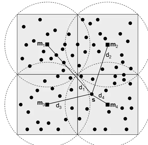
mi is the node location and ri is a predefined effective ra-dius. The formula in Eq. (13) represents a bi-square bell-shaped function that has its maximum value at mi and de-creases smoothly until it reaches zero outside the circle. To demonstrate this, a schematic diagram for the node setup is shown in Fig. 6. Within the domain of the data, four nodes,m1,· · ·,m4, are defined with a corresponding radius. In Fig. 6, ifsis located within the radius of a certain node, it gets a positive weight; otherwise, the weight is zero. Hence, S(s)= [0,0,0, S(s)].

The last component in Eq. (12) accounts for the variations of the process that has not been captured so far (Kang and

m₁ m₂

d₂

m_{3 m}

4 d₄ d₃

d₁

s

Figure 6. The observation domain with the black dots defines the

locations at which the data are available. The black little squares indicate the nodes. The weights for each locations are related to the distancesd_i. The dashed circles define the radius for each node.

Cressie, 2011). The componentζ is assumed to be an un-correlated Gaussian process with a mean zero and a variance

σ_ζ2.

Based on the model in Eq. (12), the FRK estimator is found whenηandζ are determined; i.e.,

ˆ

Y (so)=Sp(so)· ˆη+ ˆζ (so)

=Sp(so)KS06−1eZ+σ2_ζE(so=s)6−1eZ, (14)

where Sp(so)is the weighting matrix for the prediction lo-cation and6is the covariance matrix of the input data. The matrix E in Eq. (14) has a value of one ifs=so and zero elsewhere.Yˆ represents the detrended estimator.ηˆandζˆ are the optimal a posteriori estimates ofη and ζ, respectively (Braverman et al., 2011). In order to get the total value of_Yˆ

t, we calculate

ˆ

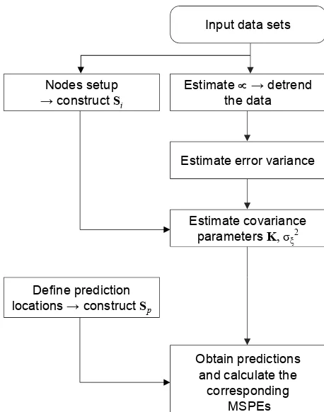
Yt(so)=T(so)· ˆα+ ˆY (so). (15) The steps followed to obtain the predictions based on the FRK method are summarized in Fig. 7. The methods to esti-mate the noise varianceσ2, the covariance matrix K, and the variance of the fine-scale signalσ_ζ2are shown in Appendix A. We classify the spatial variations of the atmospheric wa-ter vapor signal into three components: long wavelength, medium to short wavelength, and uncorrelated fine scale. Therefore, we split the water vapor signal using the linear model in Eq. (12) and use the FRK method for prediction.

Nodes setup

→ construct Si

Estimate error variance

Estimate covariance

parameters K, σ_ξ2

Input data sets

Estimate → detrend

the data

Define prediction

locations → construct Sp

Obtain predictions and calculate the

corresponding MSPEs

Figure 7. Obtaining predictions via the FRK method.

7.6 7.8 8.0 8.2 8.4 48.7

48.8 48.9 49.0 49.1 49.2 49.3 49.4

Longitude [°]

Latitude [°]

Scale1 Scale2 Scale3

Figure 8. FRK nodes or center locations of 93 basis functions at

three spatial resolutions. The first resolution is 40 km, the second resolution is 20 km, and the third resolution is 10 km.

FRK, the matrix S is constructed using the node setup shown in Fig. 8. The nodes or center locations of 93 basis functions are established at three spatial resolutions: the first resolu-tion is 40 km, the second resoluresolu-tion is 20 km, and the third resolution is 10 km. The semivariogram and the fitted spher-ical variogram model are shown in Fig. 9a, while the covari-ance matrix determined using the FRK method is shown in Fig. 9b. The predicted maps with 3 km×3 km resolution are shown in Fig. 10. Due to the lack of ground truth data that

should be used to estimate the bias in the model data, we do not add the long-wavelength component into the figures to enable unbiased comparison. We observe similar results from both ordinary kriging and fixed-rank kriging that agree with the original WRF map. The spatial correlation coeffi-cients with the corresponding WRF data are approximately 85 and 83 % for FRK and OK, respectively. When using OK, we assumed the signal to be spatially isotropic to ease the computations; therefore, the OK prediction map shows re-sults sightly different from the FRK. The most impressive point here is the computational time reported for both algo-rithms. The FRK algorithm is fast, so that it requires signif-icantly shorter time to produce the predictions. Most of the time is invested in the calculations of the covariance model parameters and constructing the matrices S and6. We imple-mented the OK algorithm such that the predictions are found iteratively. Also, to estimate a value at locations, we do not use the entire data, but only those that exist within a prede-fined radius around the prediction location. Nevertheless, the OK algorithm requires computational time with an order of magnitude higher than that required by the FRK method, on the same machine.

In the next section, we describe the extension of the FRK method for predicting the atmospheric PWV by fusing re-mote sensing data and the WRF model.

5 Data fusion for water vapor estimation

In this section, we fuse the PWV maps derived from the re-mote sensing data and WRF model. Since we classify the spatial variations of the atmospheric water vapor signal into long wavelength, medium to short wavelength, and uncor-related fine-scale components, we use the following model setup for prediction.

5.1 Model setup

PWV maps will be derived from the remote sensing data, denoted Z1, and those from the WRF model denoted Z2 with the sizesN1andN2, respectively.Z1contains the point PWV estimates from remote sensing data and Z2 contains the block WRF data. Following the SME model in Eq. (12), the two data sets can be expressed as

Z1

Z2

=

T1 T2

α+

S1 S2

η+

ζ₁

0

+

1

2

. (16)

(a) (E)

Range

Sill

Figure 9. (a) The experimental semivariogram and the fitted spherical variogram model. (b) Covariance matrix used to predict the wet delay

maps in Fig. 10.

Figure 10. Wet delay prediction map using block OK and FRK. The resolution of the grid is 3 km×3 km. A point-level wet delay map, on 23 May 2005 at 09:51 UTC, is used as input to the algorithms.

at a resolution of 3 km×3 km; therefore, the highly variable signal of water vapor is smoothed. Hence, we do not add the componentζfor the model data.

To solve the system in Eq. (11), we determine the covari-ance structure associated with each SRE model in Eq. (16), i.e.,

611=var(eZ1)=S1KS01+σζ2Vζ+σ21V1, (17)

622=var(eZ2)=eS2KeS

0

2+σ22V2, (18)

612=cov(eZ1,eZ2)=S1KeS0₂=60₂₁, (19)

whereσ_ζ2Vζ andσ2Vare diagonal covariance matrices for

ζ and, respectively. Note that when computing the cross-covariance functions 612and621, the only part of the sig-nals that is assumed correlated isη. In order to solve Eq. (11), we need not only to specify the covariance matrices of the input data, but also to find the covariance between the obser-vations and the spatial process at the prediction locations.

The covariance terms are obtained from

c1=cov(eZ1(s), Y (so)) =Sp(so)KS01(s)+σ 2

ζE(s=so); (20)

c2=cov(eZ2, Y (so))=Sp(so)KeS0₂. (21)

The matrix E in Eq. (20) has a value of one ifs=soand zero elsewhere. By solving fora1anda2in Eq. (11) and substi-tuting the results in Eq. (8), the estimatorY (ˆ so)becomes

ˆ Y (so)=

Sp(so)K

S0₁

eS0 2

+

σ_ζ2E

0

6₁₁ 6₁₂ 621 622

−1 e Z₁

e Z₂

. (22) The mean squared prediction error (MSPE) corresponding to

ˆ

Y can be obtained from

MSPE=a0₁611a1+a02622a2+2a10612a2−2a01c1−2a02c2. (23)

Using the FRK covariance model in Eq. (19) makes the matrix inversion of Eq. (22) scalable. That is, the matrix in-version can be achieved by applying a recursive block-wise inversion as follows:

A B

C D

−1

=

O1 O2 O3 O4

Table 1. Model components from point-level and areal-level data.

Point data Block data

True process Y (s) Y (Bi)= |B1i| P

s⊂Bi Y (s)

Trend T(s)α _|B1

i| P

s⊂Bi T (s)

! α

Weighting matrix S(s) eS(B_i)= _|1

Bi| P

s⊂Bi S(s)

Medium-scale signal S(s)η eS(B_i)η Fine-scale signal ζ (s) ζ (Bi)=|B1i|

P

s⊂Bi ζ (s)

Error (s) (Bi)

where

O1=A−1+A−1B(D−CA−1B)−1CA−1, O2= −A−1B(D−CA−1B)−1,

O3= −(D−CA−1B)−1CA−1, O4=(D−CA−1B)−1,

and A,B,C, and D are matrices of any size, and A and D must be square. The inversion of individual matrices in Eq. (24) is achieved by applying the formula of Sherman– Morrison–Woodbury, which is made possible due to the FRK covariance structure,

6−1_ii =(Di+SiKiS0i)−1

=D−1_i −D−1_i Si(K−1+S0iD −1

i Si)−1S0iD −1

i . (25) The computations require the inversion of the matrices K and

(K−1+S0_iD_i−1Si), where each of them has the sizer×rwith

rsignificantly smaller than the data size. Note that Diis a di-agonal matrix, for which the inversion is achieved by invert-ing the diagonal elements. Usinvert-ing the FRK covariance model makes the computational burden for the matrix inversion lin-ear with the data size (Cressie and Johannesson, 2008). 5.2 Application to the data

In this section, we build PWV maps from remote sensing and WRF model data using a spatial statistical data fusion method. The first PWV map, derived by combining GNSS and PSI, has 169 688 data points. The WRF model provides a block-level map of 1296 cells of the size 3 km×3 km. The data to be fused have different qualities, a huge size, different spatial supports, and gaps in the remote sensing data. The output grid is defined at 3 km×3 km (block-level support) and MERIS PWV maps are used for evaluation.

Following the work flow in Fig. 7, we first estimate the long wavelength trends and remove them from the data using Eq. (7). By comparing the PWV from the WRF model and

Figure 11. PWV maps from the PSI + GNSS combination and WRF

on 5 September 2005, with a linear trend subtracted from each map. PSI + GNSS provide point-level observations, while WRF generates block data with a block size of 3 km×3 km. The predictions will be obtained within the area indicated by the black box.

remote sensing data, we found it is most likely that the model data have a bias. Due to the lack of a priori information about the bias and the absence of accurate ground truth data to esti-mate it, we estiesti-matedαindependently for each data set. The centered maps are shown in Fig. 11.

loca-Table 2. Spatial correlation coefficients (CC) and rms values when comparing the prediction maps with MERIS PWV maps.

Method 5 September 2005 27 June 2005

Spatial CC rms (mm) Spatial CC rms (mm)

WRF data 0.70 1.33 0.85 0.87

Remote sensing data 0.87 0.90 0.72 1.13

Data fusion 0.91 0.82 0.86 0.92

tions is done in a similar way, either at point level or block level, depending on the output grid.

In the third step, the covariance parameters (K, σ_ζ2, σ2) are estimated from the centered dataeZ1andeZ2. The error vari-ances for both data sets, K andσ_ζ2, are estimated as described in Appendix A. Note that when the two data sets are com-bined to infer a single process, i.e., PWV, one K is estimated for all data sets.

Results

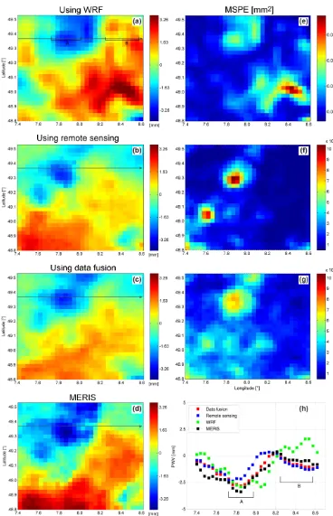
So far, all components required to produce the predictions using Eq. (22) have been obtained. In Fig. 12, we show the prediction maps obtained by applying FRK to individual data sets as well as the map obtained by data fusion. The figure also shows the MSPE maps associated with each prediction map. We compare the interpolations obtained by applying FRK to single data sets with those obtained by SSDF, and we compare both with the MERIS data. The results show that the map obtained by data fusion correlates more consistently with the map predicted only from PSI + GNSS (Table 2). In the PWV map generated by WRF, shown in Fig. 11, the area in the lower left corner shows artifacts that do not reflect the correct values of PWV as observed from the MERIS PWV map (Fig. 3c and d). Applying FRK to the WRF data does not remove these artifacts from the prediction map. How-ever, in the map obtained by the fusion of both data sets, the artifacts in the lower corner disappeared, but the corre-sponding MSPE values are large for this region. The MSPE values corresponding to the SSDF predictions are generally smaller, and we should note that in the regions of sparse ob-servations, the corresponding MSPE values tend to increase. For regions of sparse observations in the PWV map (Fig. 11), i.e., the areas in the west of the Rhine valley or in the lower right corner, the map from the WRF model contributes to im-proving the estimation of the PWV values in the prediction map. The region in the lower right corner has a higher to-pography and the wet delay values are expected to decrease, as we observe from the map of WRF. In the prediction map obtained by applying FRK to PWV from PSI and GNSS, the predicted values tend to increase since the data in this area are sparse and partially biased. By applying the SSDF approach, the data available from WRF influence the predictions such that the PWV values in this area are more reasonable, and they decrease by moving to the lower right corner. In a

sim-ilar way, the data from WRF improve the predictions in the region around 7.8◦E, 49.25◦N, where only sparse PWV data exist. The data from the model, however, affect the prediction in the lower left corner such that they are smaller than those observed in the MERIS map.

In addition, we show the PWV profiles over the line drawn horizontally at the latitude 49.37◦N in Fig. 12h. It is ob-served from the plots that the predictions made by data fusion are affected more by the data from WRF in region A, where the remote sensing data are sparse. However, in region B, the WRF data are significantly overestimated. In the prediction map made by data fusion, these data have a lower effect in than those received from the remote sensing data. The map received by applying the data fusion shows the best spatial correlation with the data from MERIS and the smallest rms value (see Table 2).

In the above example, the data from remote sensing have a more significant influence on the output. In Fig. 13, we show another example where the model highly affects the pre-dicted map. The prepre-dicted map based on model data shows a better spatial correlation and a lower uncertainty value com-pared to the map predicted using remote sensing data. In this case, the fusion map is more affected by the model data. The spatial correlation coefficients and the values of uncertainty are given in Table 2. In the first example (Fig. 12), the effect of the remote sensing data on the prediction map is signifi-cant. The other examples in Fig. 13 and Table 2 show that the model has a larger effect on the output map.

6 Conclusions and outlook

ap-Figure 12. PWV prediction and MSPE maps obtained by data fusion of PWV estimates from PSI and GNSS and maps from WRF as well

Figure 13. PWV maps from remote sensing (PSI+GNSS) and WRF model data on 27 June 2005 at 09:51 UTC as well as prediction maps

obtained by data fusion and individual data sets. The output grid has a block size of 3 km×3 km over the area indicated by the black box in

(a) and (b).

proach that attempts to solve the problems of computational complexity of huge data sets, change of support, and bias. We inferred PWV data on a grid of 3 km×3 km and com-pared the results with PWV maps inferred from MERIS data on the same grid. The results show a strong correlation be-tween data fusion maps and those maps from MERIS. The difference between both maps shows uncertainty values of

less than 1 mm, which is lower than that obtained from infer-ring data based on single sets.

Appendix A: Estimation covariance parameters

Predicting the stochastic component of the atmospheric sig-nal using kriging requires obtaining the covariance function

6and fitting a covariance model. Using the FRK covariance model, we need to estimate the matrix K, the noise variance

σ2, and the variance of the fine-scale signal σ_ζ2. The first method proposed to estimate K is called the binned method of moments (MM) (Cressie and Johannesson, 2008; Nguyen, 2009). This approach derives the empirical estimator for6

and obtains K such that|| ˆ6−6||_F is minimum, where|| · ||_F refers to the Frobenius norm.

Another approach proposed by Katzfuss and Cressie (2009) targets determination of the covariance parameters us-ing the algorithm of maximum likelihood estimation (MLE). Furthermore, they estimated the covariance parameters using the expectation–maximization (E–M) algorithm (Dempster et al., 1977) to reduce the computational burden. This algo-rithm provides estimates not only of K, but also ofσ_ζ2, where the solution for the MLEs is found iteratively. Within each it-eration the algorithm performs two steps, the expectation and the maximization. In the following, we present a description of how to obtain the maximum likelihood estimates of the covariance model parameters via the E–M algorithm.

Assume that the observations in eZ follow a multivariate

Gaussian distribution; that is,eZ∼N (0,6). Let the

param-eters of interest K and σ_ζ2be summarized in the vector 2; then, the likelihood functionL(2)is (Katzfuss and Cressie, 2009)

−2 logL(2)= −2f (eZ;2)

=log det6+eZ

0

6−1eZ+c

=log det6+ tr(6−1eZeZ

0

)+c, (A1)

wherec=(N/2)log 2πis a constant independent of2, and hence it cancels out in the maximization step. tr(·)denotes the trace operator of a square matrix, with tr(A)=Pn

i=1aii. In the expectation step of the algorithm, we calculate

Q(2;2[t])=E₂[t]{−2 logL(η,ζ;2)|eZ}, (A2)

given that

−2 logL(η,ζ;2)= log det K+ tr(K−1ηη0)+Nlogσ_ζ2

+σ_ζ−2tr(ζ ζ0)+Nlogσ2+σ−2tr(0).

Then Eq. (A2) becomes

Q(2;2[t])= −1 2

h

log det K+ tr(K−1E₂[t]{ηη0|eZ})

+Nlogσ_ζ2+σ_ζ−2tr(V_ζ−1E₂[t]{ζ ζ0|eZ}) (A3)

+Nlogσ2+σ−2tr(V−1 E₂[t]{0|eZ}) i

.

We should remind the reader that the parameters to be esti-mated here are K andσ_ζ2, whileσ2is estimated from the ro-bust semivariogram, as described later. To proceed with the

solution, we are required to quantify the conditional expec-tations in Eq. (A3). Using the standard formula required for calculating conditional expectations for multivariate normal distribution, the expectations will have the following form (Katzfuss and Cressie, 2009):

E₂[t]{ηη0|eZ} =6_η[t]+µ[_ηt]µ0[_ηt],

E₂[t]{ζ ζ0|eZ} =6

[t] ζ +µ

[t] ζ µ

0[t] ζ , with

µ_η[t]=E₂[t]{η|eZ} =K

[t]

S06t−1eZ,

µ_ζ[t]=E₂[t]{ζ|eZ} =σ_ζ2

[t]

Vζ6[t]− 1

e

Z,

6[_ηt]=cov₂[t](η|eZ)=K

[t]_−K[t]_S0₆[t]−1_SK[t] ,and

6[_ζt]=cov₂[t](ζ|eZ)=σ_ζ2

[t]

Vζ−σζ2 [t]

Vζ6[t]− 1

σ_ζ2[t]Vζ. After the expectation step, we perform a maximization step. The parameters K andσ_ζ2in Eq. (A3) should be selected such thatQ(·)is maximized. The partial derivative is taken with respect to both parameters and the result is assigned to zero. Finding the derivative here is rather simple since η andζ

do not show dependency on each other, as observed from Eq. (A3). The updating scheme of the E–M algorithm in each iteration is

K[t+1]=K[t]+K[t]S06[t]−1eZeZ 0

6[t]−1−I_NSK[t]; (A4) σζ2

[t+1] =σζ2

[t] +σζ2

[t] tr

1 N6

[t] −1 e ZeZ

0

6[t] −1−INVζ

σζ2 [t]

. (A5) We keep updating the solution until the algorithm converges. One criterion to monitor convergence is to calculate the norm of the difference between the current and last update of the vector2 (which is of sizer2+1). That means||2[t+1]−

2[t]||< bshould hold for a small enough and positive value ofb. Following Katzfuss and Cressie (2009),b is assigned a value of 10−6r2. The starting choice of K andσ_ζ2should be valid; strictly speaking, K[0]must be symmetric and positive-definite andσ_ζ2[0]must be positive; i.e., K[0]=0.9·var(eZ)Ir andσ_ζ2[0]=0.1·var(eZ).

The measurement error varianceσ2is estimated separately from the empirical semivariogram of the data. Estimating bothσ2andσ_ζ2from the data is not a trivial task. That is be-cause the nugget effect in the semivariogram reflects not only the error variance, but may also be affected by the fine-scale variance. Therefore, having information about the error dis-tribution and variance is worthwhile. In our case we estimate

σ2 using the method of a robust semivariogram (Cressie, 1993),

2γ (h)=

1 |N (h)|

P

N (h)

Z(ui)−Z(uj)

1/24

0.457+ 0.494 |N (h)|

Figure A1. Estimate of the covariance matrix K using the E–M

al-gorithm and the corresponding covariance matrix for the wet delay map from PSI + GNSS. The wet delay observations are aggregated into maps of 7×7 km2 cells before their covariance matrices are computed.

wherehis the separation distance, assuming the signal is spa-tially isotropic. To obtain an estimate ofσ2, a straight line is fitted to the estimated semivariogram at short h. Since the slope of the structure function (variogram) describing atmo-spheric turbulence is expected to vary withh, we made the line fitting based on the estimates of the first 3 km (empiri-cally defined). Let the line fit beγ (h)ˆ = ˆγ (0+)+bh; then, the estimate ofσ2is

ˆ

σ2= ˆγ (0+). (A7)

Shouldγ (ˆ 0+)have a negative value,σˆ2is set to zero.

Acknowledgements. The authors would like to thank the GNSS data providers: RENAG, RGP, Teria, and Orpheon (France), SAPOS®-Baden-Württemberg and Rheinland-Pfalz (Germany), the European Permanent Network, and IGS. We thank the ESA for the ASAR and MERIS data. We also acknowledge the ECWMF for providing the ERA-INTERIM reanalysis data.

The article processing charges for this open-access publication were covered by a Research

Centre of the Helmholtz Association.

Edited by: E. Zehe

References

Alshawaf, F., Fersch, B., Hinz, S., Kunstmann, H., Mayer, M., Thiele, A., Westerhaus, M., and Meyer, F.: Analysis of atmo-spheric signals in spaceborne InSAR – toward water vapor map-ping based on multiple sources, in: Geoscience and Remote Sensing Symposium (IGARSS), 2012 IEEE International, 1960– 1963, 2012.

Alshawaf, F., Fuhrmann, T., Knopfler, A., Luo, X., Mayer, M., Hinz, S., and Heck, B.: Accurate Estimation of Atmospheric Water Vapor Using GNSS Observations and Surface Meteoro-logical Data, IEEE T. Geosci. Remote Sens., 53, 3764–3771, doi:10.1109/TGRS.2014.2382713, 2015a.

Alshawaf, F., Hinz, S., Mayer, M., and Meyer, F. J.: Constructing accurate maps of atmospheric water vapor by combining inter-ferometric synthetic aperture radar and GNSS observations, J. Geophys. Res.-Atmos., 120, 1391–1403, 2015b.

Awan, N. K., Truhetz, H., and Gobiet, A.: Parametrization-Induced Error Characteristics of MM5 and WRF Operated in Climate Mode over the Alpine Region: An Ensemble-Based Analysis., J. Climate, 24, 3107–3123, 2011.

Bender, M., Dick, G., Wickert, J., Schmidt, T., Song, S., Gendt, G., Ge, M., and Rothacher, M.: Validation of GPS slant delays using water vapor radiometers and weather models, Meteorol. Z., 17, 807–812, 2008.

Bennitt, G. and Rupp, A.: Operational assimilation of GPS zenith total delay observations into the Met Office numerical weather prediction models, Mon. Weather Rev., 140, 2706–2719, 2012. Berg, P., Wagner, S., Kunstmann, H., and Schädler, G.: High

reso-lution regional climate model simulations for Germany: part I – validation, Clim. Dynam., 40, 401–414, 2013.

Bevis, M., Businger, S., Herring, T. A., Rocken, C., Anthes, R. A., and Ware, R. H.: GPS meteorology: remote sensing of atmo-spheric water vapor using the global positioning system, J. Geo-phys. Res.-Atmos., 97, 15787–15801, 1992.

Braverman, A., Nguyen, H., and Olsen, E.: Space-Time Data Fu-sion, Earth Science, Earth Science Technology Forum, Pasadena, California, 2011.

Braverman, A. J., Cressie, N., Katzfuss, M., Michalak, A. M., Miller, C. E., Nguyen, H., Olsen, E. T., and Wang, R.: Geosta-tistical data fusion for remote sensing applications, AGU Fall Meeting Abstracts, p. C1014, 2009.

Chen, F. and Dudhia, J.: Coupling an advanced land surface-hydrology model with the Penn State–NCAR MM5 Modeling

System. Part I: Model implementation and sensitivity, Mon. Weather Rev., 129, 569–585, 2001.

Cimini, D., Pierdicca, N., Pichelli, E., Ferretti, R., Mattioli, V., Bonafoni, S., Montopoli, M., and Perissin, D.: On the accuracy of integrated water vapor observations and the potential for miti-gating electromagnetic path delay error in InSAR, Atmos. Meas. Tech., 5, 1015–1030, doi:10.5194/amt-5-1015-2012, 2012. Collins, W. D., Rasch, P. J., Boville, B. A., Hack, J. J., McCaa, J. R.,

Williamson, D. L., Kiehl, J. T., Briegleb, B., Bitz, C., Lin, S., Zhang, M., and Dai, Y.: Description of the NCAR Community Atmosphere Model (CAM 3.0), Tech. rep., Climate And Global Dynamics Division National Center For Atmospheric Research Boulder, Colorado, 2004.

Cressie, N.: Statistics for Spatial Data, Wiley, New York, 1993. Cressie, N. and Johannesson, G.: Fixed rank kriging for very large

spatial data sets, J. Roy. Stat. Soc. B Met., 70, 209–226, 2008. Dee, D. P., Uppala, S. M., Simmons, A. J., Berrisford, P., Poli,

P., Kobayashi, S., Andrae, U., Balmaseda, M. A., Balsamo, G., Bauer, P., Bechtold, P., Beljaars, A. C. M., van de Berg, L., Bid-lot, J., Bormann, N., Delsol, C., Dragani, R., Fuentes, M., Geer, A. J., Haimberger, L., Healy, S. B., Hersbach, H., Holm, E. V., Isaksen, L., Kallberg, P., Köhler, M., Matricardi, M., McNally, A. P., Monge-Sanz, B. M., Morcrette, J.-J., Park, B.-K., Peubey, C., de Rosnay, P., Tavolato, C., Thepaut, J.-N., and Vitart, F.: The ERA-Interim reanalysis: configuration and performance of the data assimilation system, Q. J. Roy. Meteor. Soc., 137, 553–597, doi:10.1002/qj.828, 2011.

Dempster, A. P., Laird, N. M., and Rubin, D. B.: Maximum likeli-hood from incomplete data via the EM algorithm, J. Roy. Stat. Soc. B, 39, 1–38, 1977.

Ferretti, A., Prati, C., and Rocca, F.: Permanent scatterers in SAR interferometry, IEEE T. Geosci. Remote, 39, 8–20, 2001. Fersch, B. and Kunstmann, H.: Atmospheric and terrestrial

wa-ter budgets: sensitivity and performance of configurations and global driving data for long term continental scale WRF simula-tions, Clim. Dynam., 42, 2367–2396, 2014.

Fersch, B., Kunstmann, H., Devaraju, B., and Sneeuw, N.: Large scale water storage variations from regional atmospheric water budgets and comparison to the GRACE spaceborne gravimetry, J. Hydrometeorol., 13, 1589–1603, 2012.

Fischer, J. and Bennartz, R.: Retrieval of Total Water Vapour Con-tent from MERIS Measurements: Algorithm Theoretical Basis Document ; ATBD 2.4, Freie Universität Berlin, Berlin, Ger-many, 1997.

Gelfand, A. E., Zhu, L., and Carlin, B. P.: On the change of support problem for spatio-temporal data, Biostatistics, 2, 31–45, 2001. Gong, W., Meyer, F., Webley, P., Morton, D., and Liu, S.:

Perfor-mance analysis of atmospheric correction in InSAR data based on the Weather Research and Forecasting Model (WRF), in: Geo-science and Remote Sensing Symposium (IGARSS), 2010 IEEE International, 25–30 July 2010, Honolulu, Hawaii, USA, 2900– 2903, 2010.

Hanssen, R.: Radar Interferometry: Data Interpretation and Error Analysis, Kluwer Academic Publishers, Dordrecht, the Nether-lands, 2001.

Hong, S.-Y., Noh, Y., and Dudhia, J.: A new vertical diffusion pack-age with an explicit treatment of entrainment processes, Mon. Weather Rev., 134, 2318–2341, 2006.

Hooper, A., Segall, P., and Zebker, H.: Persistent scatterer interfer-ometric synthetic aperture radar for crustal deformation analysis, with application to Volcán Alcedo, Galápagos, J. Geophys. Res.-Solid Earth, 112, B07407, doi:10.1029/2006JB004763, 2007. Jade, S. and Vijayan, M.: GPS-based atmospheric precipitable water

vapor estimation using meteorological parameters interpolated from NCEP global reanalysis data, J. Geophys. Res.-Atmos., 113, D03106, doi:10.1029/2007JD008758, 2008.

Kain, J. S.: The Kain–Fritsch convective parameterization: an up-date, J. Appl. Meteorol., 43, 170–181, 2004.

Kang, E. L. and Cressie, N.: Bayesian inference for the spatial ran-dom effects model, J. Am. Stat. Assoc., 106, 972–983, 2011. Karabati´c, A., Weber, R., and Haiden, T.: Near real-time estimation

of tropospheric water vapor content from ground based GNSS data and its potential contribution to weather now-casting in Aus-tria, Adv. Space Res., 47, 1691–1703, 2011.

Katzfuss, M. and Cressie, N.: Maximum likelihood estimation of covariance parameters in the spatial-random-effects model, in: Proceedings of Joint Statistical Meetings Alexandria, American Statistical Association, 1–6 August 2009, 3378–3390, 2009. Luo, X., Mayer, M., and Heck, B.: Extended neutrospheric

mod-elling for the GNSS-based determination of high-resolution at-mospheric water vapor fields, Bol. Cien. Geod., 14, 149–170, 2008.

Massonnet, D., Rossi, M., Carmona, C., Adragna, F., Peltzer, G., Feigl, K., and Rabaute, T.: The displacement field of the Landers earthquake mapped by radar interferometry, Nature, 364, 138– 142, 1993.

Mateus, P., Nico, G., Tomé, R., Catalão, J., and Miranda, P.: Com-parison of precipitable water vapor (PWV) maps derived by GPS, SAR interferometry, and numerical forecasting models, SPIE, 7827, 14–20, 2010.

Meyer, F., Bamler, R., Leinweber, R., and Fischer, J.: A compar-ative analysis of tropospheric water vapor measurements from MERIS and SAR, in: Geoscience and Remote Sensing Sym-posium, IGARSS 2008, IEEE International, 6–11 July, 2008, Boston, Massachusetts, Vol. 4, IV-228–IV-231, 2008.

Nguyen, H.: Spatial Statistical Data Fusion for Remote Sensing Ap-plications, PhD thesis, University of California, Los Angeles, USA, 2009.

Onn, F. and Zebker, H. A.: Correction for interferometric synthetic aperture radar atmospheric phase artifacts using time series of zenith wet delay observations from a GPS network, J. Geophys. Res.-Solid Earth, 111, B09102, doi:10.1029/2005JB004012, 2006.

Pichelli, E., Ferretti, R., Cimini, D., Perissin, D., Montopoli, M., Marzano, F. S., and Pierdicca, N.: Water vapor distribution at urban scale using high-resolution numerical weather model and spaceborne SAR interferometric data, Nat. Hazards Earth Syst. Sci., 10, 121–132, doi:10.5194/nhess-10-121-2010, 2010. Prein, A. F., Langhans, W., Fosser, G., Ferrone, A., Ban, N.,

Goer-gen, K., Keller, M., Tölle, M., Gutjahr, O., Feser, F., Brisson, E., Kollet, S., Schmidli, J., van Lipzig, N. P. M., and Leung, R.: A review on regional convection-permitting climate modeling: Demonstrations, prospects, and challenges, Rev. Geophys., 53, 323–361, doi:10.1002/2014RG000475, 2015.

Rocken, C., Hove, T. V., Johnson, J., Solheim, F., Ware, R., Be-vis, M., Chiswell, S., and Businger, S.: GPS/STORM-GPS sens-ing of atmospheric water vapor for meteorology, J. Atmos. Ocean. Tech., 12, 468–478, 1995.

Skamarock, W. C. and Klemp, J. B.: A time-split nonhy-drostatic atmospheric model for weather research and fore-casting applications, J. Comput. Phys., 227, 3465–3485, doi:10.1016/j.jcp.2007.01.037, 2008.

Skamarock, W. C., Klemp, J. B., Dudhia, J., Gill, D. O., Barker, D. M., Wang, W., and Powers, J. G.: A Description of the Advance Research WRF Version 3, NCAR Technical Note NCAR/TN-468+STR, National Center for Atmospheric Research, Boulder, Colorado, USA, 2008.

Uppala, S., Dee, D., Kobayashi, S., Berrisford, P., and Simmons, A.: Towards a climate data assimilation system: status update of ERA-Interim, ECMWF Newsl., 115, 12–18, 2008.

Zebker, H. A. and Goldstein, R. M.: Topographic mapping from in-terferometric synthetic aperture radar observations, J. Geophys. Res.-Solid Earth, 91, 4993–4999, 1986.

Zebker, H. A., Rosen, P. A., Goldstein, R. M., Gabriel, A., and Werner, C. L.: On the derivation of coseismic displacement fields using differential radar interferometry: the Landers earthquake, J. Geophys. Res.-Solid Earth, 99, 19617–19634, 1994.