www.hydrol-earth-syst-sci.net/19/2755/2015/ doi:10.5194/hess-19-2755-2015
© Author(s) 2015. CC Attribution 3.0 License.
Technical Note: A simple generalization
of the Brutsaert and Nieber analysis
T. L. Chor1and N. L. Dias2
1Graduate Program in Environmental Engineering (PPGEA), Federal University of Paraná, Curitiba, Brazil 2Department of Environmental Engineering, UFPR, Curitiba, Brazil
Correspondence to: N. L. Dias ([email protected])
Received: 12 October 2014 – Published in Hydrol. Earth Syst. Sci. Discuss.: 12 November 2014 Revised: 21 May 2015 – Accepted: 22 May 2015 – Published: 16 June 2015
Abstract. The Brutsaert and Nieber (1977) analysis is a well-known method that can estimate soil parameters given dis-charge data for some aquifers. It has been used for several cases where the observed late-time behavior of the recession suggests that the water stream that is adjacent to the aquifer has nonzero depth. However, its mathematical formulation is, strictly speaking, not capable of reproducing these real-case scenarios since the early time behavior is based on a solution for which the aquifer stream has zero depth (Polubarinova-Kochina, 1962). We propose a simple generalization for the Brutsaert and Nieber (1977) method that takes into consider-ation the depth of the adjacent water stream. The generaliza-tion is based on already available solugeneraliza-tions by Polubarinova-Kochina (1962), Chor et al. (2013) and Dias et al. (2014) and can be readily implemented with little effort. The original and proposed equations are tested against numerical simula-tions of the full nonlinear Boussinesq equation. A sensitivity analysis shows that the modification can have significant im-pact on the predicted values of both the drainable porosity and the saturated hydraulic conductivity.
1 Introduction
The Brutsaert and Nieber (1977) analysis (from now on ferred to as BN77) has been widely used in hydrologic re-search to estimate aquifer parameters given some discharge data. This technique is based on “state-space”-like plots of
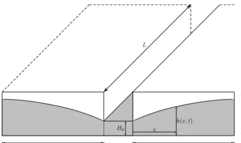
Q×dQ/dt, whereQ(t )is the aquifer discharge as a function of time. It is based on solutions for the Boussinesq equation for groundwater flow applied to a system as the one presented in Fig. 1, which shows a water channel of lengthLwith one
aquifer of length B on each side. Traditionally three solu-tions of the Boussinesq nonlinear partial differential equa-tion for groundwater flow (Boussinesq, 1903) are considered for this method, which are the three solutions proposed by BN77. Solution (i) was originally given as an incomplete se-ries by Polubarinova-Kochina (1962) (the complete set of co-efficients was given by Chor et al. (2013)) for a semi-infinite aquifer that deals with early-time behavior as
h(x, t )=H
∞
X
n=0
bn x √
4Dt 3n+1
2
, (1)
where the coefficientsbnare given by a recurrence relation (Chor et al., 2013),D=H k0/neandxis the horizontal
dis-tance. Solution (ii) is the exact solution provided by Boussi-nesq (1904) for a finite aquifer, which is adequate for later times. It is given by
h(x, t )=F (x) 1 ˆ
at+1, (2)
whereF (x)is defined from the incomplete beta function and
ˆ
ais a constant coefficient.
Solution (iii) is the linearized solution provided by Boussi-nesq (1903) (also appropriate for late-time behavior) which is given by
h(x, t )=H0+ 4
π(H−H0)
∞
X
n=1,3,5...
1
nsin
π nx
2B
exp
−π
2n2k 0pH 4neB2 t
. (3)
b
L
H0
H
B B
x
[image:2.612.49.287.64.205.2]h(x, t)
Figure 1. Schematic of a watershed of simple geometry during a hydrologic recession.
From the aforementioned solutions, only Solution (iii) is able to deal with nonzero water-stream depths (H0) adjacent to the aquifer (of initial water table heightH). Recently, So-lution (i) – from now on we call “SoSo-lution (i)” any soSo-lution for a semi-infinite aquifer where discharge is occurring – has been generalized by Chor et al. (2013) and Dias et al. (2014). The work by Dias et al. (2014) is of particular importance for us because it extends the early-time behavior to cases where the stream depth is different from zero.
Since BN77, many changes and improvements have been suggested (for detailed reviews, see Rupp and Selker, 2006, and Troch et al., 2013) but its main insight remains the same: that one should look at the rate of discharge as a function of discharge, or, mathematically (for the case of a power law),
dQ
dt = −αQ
β, (4)
where Q is the water discharge, t is time and α and β
are calibrated coefficients which can be compared to the predictions from the abovementioned analytical solutions by Polubarinova-Kochina (1962), Boussinesq (1903) and Boussinesq (1904), among many others (Rupp and Selker, 2006).
If one wishes to estimate only the soil hydraulic con-ductivityk0 and the drainable porosityne, two of the three
aforementioned solutions can be used. In this work, the so-lutions used are the ones by Polubarinova-Kochina (1962), Dias et al. (2014), and Boussinesq (1903). However, the so-lution by Polubarinova-Kochina (1962) is only valid for the case H0=0: it is therefore important to assess how much this assumption affects the estimate ofk0and ofnefor cases where it does not hold.
From the long list of solutions of the Boussinesq equation that are used for BN77’s method, very few takeH0into con-sideration (from the list of 13 equations presented by Rupp and Selker (2006), only 2 haveH0as a parameter), so it is safe to say that the approximation of zero water level depth has not been thoroughly studied.
Although the BN77 method has been the focus of many studies for over 40 years, the subject is not, by any means, ex-hausted. Among recent findings is the work by Bogaart et al. (2013), which shows that, for sloping aquifers, it is possi-ble to find aβcoefficient of zero – something that until then had not been found by any other work and that was again found by Hogarth et al. (2014). Recent uses of this equation include the linking of geological and geomorphological fea-tures to hydrological behavior (Mutzner et al., 2013; Vannier et al., 2014) and the definition of good engineering practices for the robust calibration of parsimonious models (Melsen et al., 2014).
Several considerations related to the complexities of real watersheds as well as the actual physical mechanisms through which baseflow is produced and routed through the watershed raise criticism on the applicability of the BN77 recession analysis. A short, and by no means exhaustive, list of such considerations includes the effect of steep hillslopes and vertical inhomogeneity ofk0, horizontal inhomogeneity (variation of hydraulic properties within the watershed), dif-ficulties in the identification ofαandβin Eq. (4) due to noisy data, geomorphological effects, etc. (Troch et al., 2013). Spa-tial heterogeneity appears to be particularly important and its effects were thoroughly investigated by Harman et al. (2009). This latter work shows (in a very analytical manner) that het-erogeneity alone can give rise to different values of the ex-ponentβ. The values of the exponents observed in real data, however, are such that they can be explained by either the hydraulics of the aquifer or by horizontal heterogeneity (Har-man et al., 2009, Fig. 9).
The usefulness of recession analysis in hydrology, how-ever, seems indisputable, as well as the validity of the Boussi-nesq model in partly explaining hydrological recessions: the Boussinesq model has proved able to include realistic effects while being kept relatively simple, and remains an important tool in obtaining representative parameters for hydrological and land-surface models at the catchment scale (Pauwels and Troch, 2010; Troch et al., 2013). As such, it is reasonable to expect recession analysis and the Boussinesq model to play important roles in future progress towards improved predic-tive capabilities in hydrology.
It is beyond the scope of this article to explore all the con-siderations mentioned above. Instead, we concentrate on a single effect that has not been given much attention (H06=0) and study it with a simple mathematical model that allows its importance to be assessed clearly and separately from other effects. This is in line with a systematic approach to iden-tify inconsistencies between the theoretical models and field conditions (Pauwels and Troch, 2010, Sect. 4). Our approach using numerical solutions follows many other similar works on hydrological recessions (van de Giesen et al., 2005; Rupp and Selker, 2006; Bogaart et al., 2013)
implementation of Solution (i) with existing solutions in or-der to investigate the effects of the depth of the adjacent water stream into the estimation of the drainable porosity and sat-urated hydraulic conductivity. This generalized implementa-tion is later shown to considerably improve the estimaimplementa-tion of the hydraulic conductivity and drainable porosity in nu-merically generated data. This result suggests that this new formulation of the BN77 analysis could potentially be useful for obtainingk0andne in man-made drainage systems and
improving simulations of drainage and water table dynam-ics from hypothetical hillslopes and for better understanding single hillslope processes, where the BN77 analysis is more likely to succeed (Troch et al., 2013, Sect. 4.3).
2 Generalization of the early-time equation
Letξdenote the Boltzmann variable for the one-dimensional Boussinesq equation (Chor et al., 2013; Dias et al., 2014),
ξ(x, t )=√x
4Dt, (5)
whereD=H k0/ne, andφdenotes a normalized water table
height,
φ= h
H, (6)
whereh(x,t) is the water table height,x is the horizontal distance from the water stream andtis time. Under the above change of variables, the Boussinesq equation is reduced to the dimensionless ordinary differential equation
d dξ
φdφ
dξ
+2ξdφ
dξ =0 (7)
together with the boundary conditions φ(0)=φ0 and
φ (∞)=1. Due to the second boundary condition, the solu-tion is only valid for the initial phase of aquifer drawdown. Forφ0=0, as already noted, the solution by Polubarinova-Kochina (1962) suffices for the BN77 analysis; forφ06=0, a series solution of the form
φ (ξ )=
∞
X
n=0
anξn (8)
has been proposed by Dias et al. (2014), with a recursion relation for thean’s. An important result in that work is an empirical equation, fitted to numerically obtained values of
a1 in the series above, for the value ofψ0, defined below. This is given as Eq. (16) in the present work.
Let us also define
ψ≡φdφ
dξ, (9)
which we apply to Darcy’s law, along with Eqs. (5) and (6) to obtain
q(x, t )=H
3/2(n
ek0)1/2 2
ψ (ξ(x, t ), H0/H )
t1/2 , (10)
whereq(x,t) is the flow rate per unit width at any pointx
of the aquifer. Since we are interested in the aquifer–stream interaction, we setx=0, which produces
q(t )=H
3/2(nek 0)1/2 2
ψ (ξ=0, H0/H )
t1/2
=H
3/2(n
ek0)1/2 2
ψ0(φ0)
t1/2 , (11)
whereψ0≡ψ (ξ=0) andφ0≡H0/H.
The value ofψ0, as far as we know, cannot be obtained an-alytically and is generally obtained numerically or by means of approximations: its calculation will be dealt with later. For now, it suffices to note thatψ0 is a function ofφ0as given above.
Writing dQ/dt= −α1Qβ1 , where the subscript 1 indi-cates the early-time solution, andQ=2L q is the flow per unit length taken over the total length (L) of the tributary and main channel sections upstream from the gaging station, with
qas in Eq. (11), yieldsβ1=3 and
α1=
h
2H3k0ne(ψ0(φ0))2L2
i−1
. (12)
Equation (12) is generally used with the assumption of
H0=0, which yields ψ0(0)=90≈0.6642, which (substi-tuting back into Eq. 12) gives the well-known Eq. (18b) of BN77.
However, often the value ofH0 is not small enough in comparison with H in order for this approximation to be valid (Munster et al., 1996; Serrano and Workman, 1998; Barlow et al., 2000; Peterson and Connelly, 2001; Langhoff et al., 2006; Ha et al., 2008; Sena and de Melo, 2012). In these cases the misplaced assumption could lead to biased estimates ofk0andne. These latter errors depend not only
on the determination ofα1 but also on the late-time equa-tions chosen and on the determination of the constants for that solution.
0.0 0.2 0.4 0.6 0.8 1.0 1.2
0.0 0.1 0.2 0.3 0.4 0.5 0.6 0.7 0.8 0.9 1.0
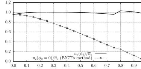
[image:4.612.310.546.68.185.2]φ0 k0(φ0)/k0 k0(φ0= 0)/k0(BN77's method)
Figure 2. Comparison between the saturated hydraulic conductivity
k0as estimated by the original BN77 analysis (dotted line and
sym-bols) and the method proposed here (solid line) – both normalized by the real valuek0used to numerically generate the discharge data
and varying against the normalized water height at the originφ0.
3 Comparison between both approaches
We dedicate this section to the estimation of the errors that arise by assuming that the stream depthH0is zero. For that purpose we take as a late-time equation the solution of the linearized Boussinesq equation, given by Eq. (3), which pre-dictsβ2=1 and
α2=
π2k0pH L2
neA2
, (13)
whereAis the area of the watershed, approximated by 2B L. Solution of Eqs. (13) and (12) gives, forneandk0,
ne=
p
2
1/2 π
H ψ0A
(α2α1)−1/2 (14)
and
k0=
A √
2pH2L2π ψ 0
α
2
α1
1/2
. (15)
In this formulation we assume both ψ0 and p to be functions of φ0=H0/H, so we have ψ0(φ0) and
p(φ0), as was previously emphasized. We also assume that
p(φ0)=(1−p0) φ0+p0, where p0=0.3465, based on the fact thatp=0.3465 forH0=0 (Brutsaert and Lopez, 1998). SettingH0=0 (and thereforeφ0=0) in this model will yield exactly the same equations as presented by Brutsaert and Lopez (1998).
To obtainψ0(φ0)we use the approximation provided by Eq. (14) of Dias et al. (2014), since it is sufficiently accurate and simple to program, viz.
ψ0(φ0)≈
90d+aφ0b 1 d
1−φ0c 1+f φ0ge, (16) witha=0.733841,b=0.999223,c=0.98359,d=2.94568,
e=0.186587,f=0.966673, andg=0.93347. As explained in Dias et al. (2014), even after a general recursion relation
0.0 0.2 0.4 0.6 0.8 1.0 1.2
0.0 0.1 0.2 0.3 0.4 0.5 0.6 0.7 0.8 0.9 1.0
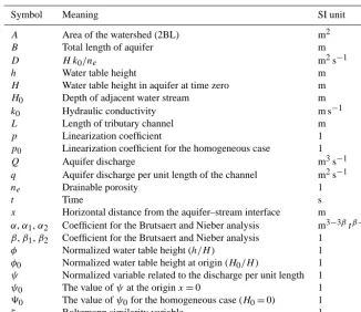
φ0 ne(φ0)/ne
ne(φ0= 0)/ne(BN77's method)
Figure 3. Comparison between the drainable porosityne as
esti-mated by the original BN77 analysis (dotted line and symbols) and the method proposed here (solid line) – both normalized by the real valueneused to numerically generate the discharge data and
vary-ing against the normalized water height at the originφ0.
for thean’s in Eq. (8) has been obtained, the values of thean’s
still cannot be obtained analytically, essentially because the series’ radius of convergence is limited so that the boundary conditionφ (∞)=1 cannot be imposed analytically. Instead, they must be obtained numerically with the aid of numer-ical solutions of Eq. (7). The coefficients above have been obtained in Dias et al. (2014) by curve fitting with a large number of numerical solutions.
In order to compare both approaches, we have solved nu-merically the original Boussinesq equation (in x andt) to model the system depicted in Fig. 1 and generated synthetic discharge data for different values ofH0< H. We then ap-plied the original BN77 method to these data, as well as the generalized method we propose here. With this analysis we can quantify the error of both methods in order to determine their accuracy.
Figures 2 and 3 show the results fork0andne, respectively,
for increasing values ofφ0, plotted against the true values
k0 andne. As can be seen, thek0estimate using the origi-nal equations remains close to the true value up toφ0=0.4 approximately. Furthermore, there is a more or less linear trend inneestimated with the original equations all the way
fromφ0=0. Both differ considerably from the truth for large values ofφ0 (φ0>0.4 for k0andφ0>0.2 forne,
approxi-mately). On the other hand, our Eqs. (15) and (14) give esti-mated values ofk0andnethat differ very little from the true ones for the wholeφ0range, and as such represent a consid-erable improvement over the original equations.
The small kinks betweenφ0=0.7 andφ0=0.8 are an arti-fact of the choice of the range of the streamflowQfor fitting
α1andα2used in the recession analysis. This (to the best of our knowledge) is still a subjective part of the BN77 analysis: the ranges were chosen to fit the recession plots dQ/dt×Q
4 Conclusions
We have given an expression for early time aquifer discharge that generalizes the broadly used Eq. (18) of Brutsaert and Nieber (1977) for cases whereH0is not small enough com-pared withHto makeφ0=0 a valid approximation and com-pared the results to the original BN77 method. The main mo-tivation for this approach was to investigate the effects of this assumption on the determination of the saturated hydraulic conductivity k0 and drainable porosityne. This
generaliza-tion, given mainly by Eq. (12), is easily applicable and re-quires virtually no change in the original theory presented by BN77.
The comparisons presented in Figs. 2 and 3 suggest that the BN77 estimates of the hydraulic conductivityk0 under-estimate the “true” numerical value more and more asφ0 in-creases. This under-estimation is particularly large whenH0 is above 40 % the value ofH (φ0>0.4). The same behav-ior is observed with the estimation of the drainable porosity
ne, with the under-estimation being specially large for H0 greater than 20 % the value of H (φ0>0.2). On the other hand, the method presented here deviates very little from the “true” numerical values in both cases and for any value of
Appendix A: List of symbols
Table A1. List of symbols used throughout the article.
Symbol Meaning SI unit
A Area of the watershed (2BL) m2
B Total length of aquifer m
D H k0/ne m2s−1
h Water table height m
H Water table height in aquifer at time zero m
H0 Depth of adjacent water stream m
k0 Hydraulic conductivity m s−1
L Length of tributary channel m
p Linearization coefficient 1
p0 Linearization coefficient for the homogeneous case 1
Q Aquifer discharge m3s−1
q Aquifer discharge per unit length of the channel m2s−1
ne Drainable porosity 1
t Time s
x Horizontal distance from the aquifer–stream interface m
α,α1,α2 Coefficient for the Brutsaert and Nieber analysis m3−3βtβ−2
β,β1,β2 Coefficient for the Brutsaert and Nieber analysis 1
φ Normalized water table height (h/H) 1
φ0 Normalized water table height at origin (H0/H) 1
ψ Normalized variable related to the discharge per unit length 1
ψ0 The value ofψat the originx=0 1
90 The value ofψ0for the homogeneous case (H0=0) 1
Acknowledgements. We would like to thank Ailín Ruiz de Zárate
for many discussions on the solutions of the Boussinesq equation.
Edited by: S. Schymanski
References
Barlow, P., DeSimone, L., and Moench, A.: Aquifer response to stream-stage and recharge variations, II. Convolution method and applications, J. Hydrol., 230, 211–229, doi:10.1016/S0022-1694(00)00176-1, 2000.
Bogaart, P. W., Rupp, D. E., Selker, J. S., and van der Velde, Y.: Late-time drainage from a sloping Boussinesq aquifer, Water Re-sour. Res., 49, 7498–7507, doi:10.1002/2013WR013780, 2013. Boussinesq, J.: Sur le débit, en temps de sécheresse, d’une source
alimentée par une nappe d’eaux d’infiltration, C. R. Hebd. Seanc. Acad. Sci. Paris, 23, 252–260, 1903.
Boussinesq, J.: Recherches théoriques sur l’écoulement des nappes d’eau infiltrées dans le sol et sur le débit des sources, J. Math. Pures Appl., 10, 5–78, 1904.
Brutsaert, W. and Lopez, J. P.: Basin-scale geohydrologic drought flow features of riparian aquifers in the southern Great Plains, Water Resour. Res., 34, 233–240, 1998.
Brutsaert, W. and Nieber, J. L.: Regionalized Drought Flow Hydro-graphs From a Mature Glaciated Plateau, Water Resour. Res., 13, 637–643, 1977.
Chor, T., Dias, N. L., and de Zárate, A. R.: An exact se-ries and improved numerical and approximate solutions for the Boussinesq equation, Water Resour. Res., 49, 7380–7387, doi:10.1002/wrcr.20543, 2013.
Dias, N. L., Chor, T. L., and Zárate, A. R.: A semi-analytical so-lution for the Boussinesq equation with nonhomgeneous con-stant boundary conditions, Water Resour. Res., 50, 6549–6556, doi:10.1002/2014WR015437, 2014.
Ha, K., Koh, D.-C., Yum, B.-W., and Lee, K.-K.: Estimation of river stage effect on groundwater level, discharge, and bank storage and its field application, Geosci. J., 12, 191–204, doi:10.1007/s12303-008-0020-y, 2008.
Harman, C. J., Sivapalan, M., and Kumar, P.: Power law catchment-scale recessions arising from heterogeneous lin-ear small-scale dynamics, Water Resour. Res., 45, w09404, doi:10.1029/2008WR007392, 2009.
Hogarth, W. L., Li, L., Lockington, D. A., Stagnitti, F., Parlange, M. B., Barry, D. A., Steenhuis, T. S., and Parlange, J.-Y.: Ana-lytical approximation for the recession of a sloping aquifer, Wa-ter Resour. Res., 50, 8564–8570, doi:10.1002/2014WR016084, 2014.
Kan, A.: Estimativa de Evapotranspiração Real com Base na Análise de Recessão dos Hidrogramas, Ph.D. thesis, Programa de Pós Graduação em Métodos Numéricos, Universidade Fed-eral do Paraná, Curitiba, 2005.
Langhoff, J. H., Rasmussen, K. R., and Christensen, S.: Quan-tification and regionalization of groundwater-surface water in-teraction along an alluvial stream, J. Hydrol., 320, 342–358, doi:10.1016/j.jhydrol.2005.07.040, 2006.
Melsen, L. A., Teuling, A. J., van Berkum, S. W., Torfs, P. J. J. F., and Uijlenhoet, R.: Catchments as simple dynamical sys-tems: A case study on methods and data requirements for parameter identification, Water Resour. Res., 50, 5577–5596, doi:10.1002/2013WR014720, 2014.
Munster, C., Mathewson, C., and Wrobleski, C.: The Texas A&M University Brazos River Hydrogeologic Field Site, Environ. Eng. Geosci., 2, 517–530, 1996.
Mutzner, R., Bertuzzo, E., Tarolli, P., Weijs, S. V., Nicotina, L., Ceola, S., Tomasic, N., Rodriguez-Iturbe, I., Parlange, M. B., and Rinaldo, A.: Geomorphic signatures on Brutsaert base flow recession analysis, Water Resour. Res., 49, 5462–5472, doi:10.1002/wrcr.20417, 2013.
Pauwels, V. R. N. and Troch, P. A.: Estimation of aquifer lower layer hydraulic conductivity values through base flow hydro-graph rising limb analysis, Water Resour. Res., 46, W03501, doi:10.1029/2009WR008255, 2010.
Peterson, R. E. and Connelly, M. P.: Zone of Interaction Be-tween Hanford Site Groundwater and Adjacent Columbia River, Tech. Rep. PNNL-13674, Pacific Northwest National Labora-tory, Richland, Washington, 2001.
Polubarinova-Kochina, P. Y.: Theory of Ground Water Movement, Princeton University Press, Princeson, NJ, 507 pp., 1962. Rupp, D. E. and Selker, J. S.: On the use of the Boussinesq equation
for interpreting recession hydrographs from sloping aquifers, Water Resour. Res., 42, W12421, doi:10.1029/2006WR005080, 2006.
Sena, C. and de Melo, M. T. C.: Groundwater-surface water inter-actions in a freshwater lagoon vulnerable to anthropogenic pres-sures (Pateira de Fermentelos, Portugal), J. Hydrol., 466, 88–102, doi:10.1016/j.jhydrol.2012.08.006, 2012.
Serrano, S. E. and Workman, S. R.: Modeling transient stream/aquifer interaction with the non-linear Boussinesq equa-tion and its analytical soluequa-tion, J. Hydrol., 206, 245–255, doi:10.1016/S0022-1694(98)00111-5, 1998.
Troch, P. A., Berne, A., Bogaart, P., Harman, C., Hilberts, A. G. J., Lyon, S. W., Paniconi, C., Pauwels, V. R. N., Rupp, D. E., Selker, J. S., Teuling, A. J., Uijlenhoet, R., and Ver-hoest, N. E. C.: The importance of hydraulic groundwater the-ory in catchment hydrology: The legacy of Wilfried Brutsaert and Jean-Yves Parlange, Water Resour. Res., 49, 5099–5116, doi:10.1002/wrcr.20407, 2013.
van de Giesen, N., Steenhuis, T. S., and Parlange, J.-Y.: Short- and long-time behavior of aquifer drainage af-ter slow and sudden recharge according to the linearized Laplace equation, Adv. Water Resour., 28, 1122–1132, doi:10.1016/j.advwatres.2004.12.002, 2005.