Reducing structural uncertainty in conceptual hydrological modelling in the semi arid Andes

www.hydrol-earth-syst-sci.net/19/2295/2015/ doi:10.5194/hess-19-2295-2015

© Author(s) 2015. CC Attribution 3.0 License.

Reducing structural uncertainty in conceptual hydrological

modelling in the semi-arid Andes

P. Hublart1,4, D. Ruelland2, A. Dezetter3, and H. Jourde1

1_{UM2 – UMR HydroSciences Montpellier, Place E. Bataillon, 34395 Montpellier CEDEX 5, France} 2_{CNRS – UMR HydroSciences Montpellier, Place E. Bataillon, 34395 Montpellier CEDEX 5, France} 3_{IRD – UMR HydroSciences Montpellier, Place E. Bataillon, 34395 Montpellier CEDEX 5, France} 4_{Centro de Estudios Avanzados en Zonas Áridas (CEAZA), Raúl Bitrán s/n, La Serena, Chile} Correspondence to: P. Hublart ([email protected]) and D. Ruelland ([email protected])

Received: 14 August 2014 – Published in Hydrol. Earth Syst. Sci. Discuss.: 31 October 2014 Revised: 16 March 2015 – Accepted: 15 April 2015 – Published: 13 May 2015

Abstract. The use of lumped, conceptual models in hydro-logical impact studies requires placing more emphasis on the uncertainty arising from deficiencies and/or ambiguities in the model structure. This study provides an opportunity to combine a multiple-hypothesis framework with a multi-criteria assessment scheme to reduce structural uncertainty in the conceptual modelling of a mesoscale Andean catch-ment (1515 km2) over a 30-year period (1982–2011). The modelling process was decomposed into six model-building decisions related to the following aspects of the system be-haviour: snow accumulation and melt, runoff generation, re-distribution and delay of water fluxes, and natural storage ef-fects. Each of these decisions was provided with a set of al-ternative modelling options, resulting in a total of 72 compet-ing model structures. These structures were calibrated uscompet-ing the concept of Pareto optimality with three criteria pertaining to streamflow simulations and one to the seasonal dynamics of snow processes. The results were analyzed in the four-dimensional (4-D) space of performance measures using a fuzzy c-means clustering technique and a differential split sample test, leading to identify 14 equally acceptable model hypotheses. A filtering approach was then applied to these best-performing structures in order to minimize the overall uncertainty envelope while maximizing the number of en-closed observations. This led to retain eight model hypothe-ses as a representation of the minimum structural uncertainty that could be obtained with this modelling framework. Future work to better consider model predictive uncertainty should include a proper assessment of parameter equifinality and

data errors, as well as the testing of new or refined hypothe-ses to allow for the use of additional auxiliary observations.

1 Introduction

Conceptual catchment models based on the combination of several interconnected stores are popular tools in flood fore-casting and water resources management (e.g. Jakeman and Letcher, 2003; Xu and Singh, 2004). The main rationale be-hind this success lies in the fact that relatively simple struc-tures with low data and computer requirements generally out-weigh the performance of far more complex physically based models (e.g. Michaud and Sorooshian, 1994; Refsgaard and Knudsen, 1996; Kokkonen and Jakeman, 2001). Also, most water management decisions are made at operational scales having much more to do with catchment-scale administra-tive considerations than with our understanding of fine-scale processes. As a result, conceptual models are being increas-ingly used to evaluate the potential impacts of climate change on hydrological systems (e.g. Minville et al., 2008; Ruelland et al., 2012) and freshwater availability (e.g. Milano et al., 2013; Collet et al., 2013).

calibra-tion process. More than a lack of physical background, this practice reveals a misunderstanding about how such mod-els should be based on physics (Kirchner, 2006; Blöschl and Montanari, 2010). Hydrological systems are not structureless things composed of randomly distributed elements, but rather self-organizing systems characterized by the emergence of macroscale patterns and structures (Dooge, 1986; Sivapalan, 2005; Ehret et al., 2014). As such, the reductionist idea that catchments can be understood by merely aggregating (up-scaling) fine-scale mechanistic laws is generally misleading (Dooge, 1997; McDonnell et al., 2007). Self-organization at the catchment scale means that new hydrologic relationships with fewer degrees of freedom have to be envisioned (e.g. McMillan, 2012a). Yet, finding simplicity in complexity does not imply that simple models available in the literature can be used as ready-made engineering tools with little or no con-sideration for the specific features of each catchment (Wain-wright and Mulligan, 2004; Savenije, 2009). As underlined by Kirchner (2006), it is important to ensure that the “right answers” are obtained for the “right reasons”. In the case of poorly defined systems where physically oriented inter-pretations can only be sought a posteriori to check for the model realism, this requires placing more emphasis on the uncertainty arising from deficiencies and/or ambiguities in the model structure than is currently done in most hydrolog-ical impact studies.

Structural uncertainty can be described in terms of inad-equacy and non-uniqueness. Model inadinad-equacy arises from the many simplifying assumptions and epistemic errors made in the selection of which processes to represent and how to represent them. It reflects the extent to which a given model differs from the real system it is intended to represent. In practice, this results in the failure to capture all relevant as-pects of the system behaviour within a single model struc-ture or parameter set. A common way of addressing this source of uncertainty is to adopt a top-down approach to model-building (Jothityangkoon et al., 2001; Sivapalan et al., 2003), in which different models of increasing complexity are tested to determine the adequate level of process rep-resentation. Where fluxes and state variables are made ex-plicit, alternative data sources (other than streamflow) such as groundwater levels (Seibert, 2000; Seibert and McDon-nell, 2002), tracer samples (Son and Sivapalan, 2007; Birkel et al., 2010; Capell et al., 2012) or snow measurements (Clark et al., 2006; Parajka and Blöschl, 2008), can also be used to improve the internal consistency of model struc-tures. Additional criteria can then be introduced in relation to these auxiliary data or to specific aspects of the hydro-graph (driven vs. non-driven components, rising limb, reces-sion limbs, etc.). In this perspective, multi-criteria evaluation techniques based on the concept of Pareto-optimality pro-vide an interesting way to both reduce and quantify structural inadequacy (Gupta et al., 1998; Boyle et al., 2000; Efstra-tiadis and Koutsoyiannis, 2010). A parameter set is said to be Pareto-optimal if it cannot be improved upon without

degrad-ing at least one of the objective criteria. In general, meandegrad-ing- meaning-ful information on the origin of model deficiencies can be derived from the mapping of Pareto-optimal solutions in the space of performance measures (often called the Pareto front) and used to discriminate between several rival structures (Lee et al., 2011). Further, the Pareto set of solutions obtained with a given model is commonly used to generate simulation en-velopes (hereafter called “Pareto-enen-velopes” for the sake of brevity) representing the uncertainty associated with struc-tural errors (i.e. model inadequacy).

semi-Figure 1. The Claro River basin at Rivadavia (1515 km2) in Chile: topography and mean annual precipitation and temperature from 1982 to 2011 (based on Ruelland et al., 2014). Several of the stations used in this study were located outside the catchment and therefore are not displayed on the following maps.

arid regions (e.g. Clark et al., 2008). Moreover, several of these studies have insisted on the need for multiple crite-ria related to different aspects of the system’s behaviour in order to improve the usefulness of MMFs. Yet, most of the time these additional criteria or signatures were not used to guide model development or constrain calibration but rather as posterior diagnostics in validation (see Kavetski and Feni-cia, 2011). Thus, the potential benefits of using the con-cept of Pareto-efficiency to constrain model development and help differentiate between numerous competing hypotheses remain largely unexplored in the current literature devoted to MMFs. Also, very few studies have included alternative conceptual representations of snow processes in their modu-lar frameworks (e.g. Smith and Marshall, 2010), even though snowmelt may have played a significant role in several cases (Clark et al., 2008; Staudinger et al., 2011).

Addressing these issues is of particular importance in the case of arid to semi-arid Andean catchments such as those found around 30◦S. The Norte Chico region of Chile, in par-ticular, has been identified as being highly vulnerable to cli-mate change impacts in a number of recent reports (IPCC, 2013) and studies (e.g. Souvignet et al., 2010; Young et al., 2010). Yet, very few catchments in this region have been studied intensively enough to provide reliable model simula-tions, often with no estimation of the surrounding uncertainty (Souvignet, 2007; Ruelland et al., 2011; Vicuña et al., 2011; Hublart et al., 2013). This study is the first step of a larger research project, whose final aim is to assess the capacity to meet current and future irrigation water requirements in a mesoscale catchment of the Norte Chico region. The ob-jective here is to provide a set of reasonable model struc-tures that can be used for the hydrological modelling of the catchment. To achieve this goal, a MMF was developed and combined with a multi-criteria optimization framework using streamflow and satellite-based snow cover data.

2 Study area

2.1 General site description

The Claro River catchment is a semi-arid, mountainous catchment located in the northeastern part of the Coquimbo region, in north-central Chile (Fig. 1). It drains an area of approximately 1515 km2, characterized by high elevations ranging from 820 m a.s.l. at the basin outlet (Rivadavia) to over 5500 m a.s.l. in the Andes Cordillera. The topography is dominated by a series of generally north-trending, fault-bounded mountain blocks interspersed with a few steep-sided valleys.

The underlying bedrock consists almost entirely of granitic rocks ranging in age from Pennsylvanian to Oligocene and locally weathered to saprolite. Above 3000 m, repeated glaciations and the continuous action of frost and thaw throughout the year have caused an intense shattering of the exposed rocks (Caviedes and Paskoff, 1975), leaving a landscape of bare rock and screes almost devoid of soil.

originates from a number of small tributaries flowing either permanently or seasonally in the mountains.

2.2 Hydro-climatic data

In order to represent the hydro-climatic variability of the catchment, a 30-year period (1982–2011) was chosen ac-cording to data availability and quality. Precipitation and temperature data were interpolated based on 12 and 8 stations, respectively (Fig. 1), using the inverse distance weighted method on a 5 km×5 km grid. Since very few mea-surements were available outside the river valleys, elevation effects on precipitation and temperature distribution were considered using the Shuttle Radar Topography Mission dig-ital elevation model (Fig. 1). In a previous study, Ruelland et al. (2014) examined the sensitivity of the GR4j hydrolog-ical model to different ways of interpolating climate forc-ing on this basin. Their results showed that a data set based on a constant lapse rate of 6.5◦C km−1for temperature and no elevation effects for precipitation provided slightly better simulations of the discharge over the last 30 years. However, since the current study also seeks to reproduce the seasonal dynamics of snow accumulation and melt, it was decided to rely on a mean monthly orographic gradient estimated from the precipitation observed series (Fig. 1). Potential evapo-transpiration (PE) was computed using the following formula proposed by Oudin et al. (2005):

PE=Re λρ ·

T+K2 K1

if T+K2>0 else PE=0, (1) where PE is the rate of potential evapotranspiration (mm d−1), Re is the extraterrestrial radiation (MJ m−2d−1), λis the latent heat flux (2.45 MJ kg−1),ρis the density of wa-ter (kg m−3), T is the mean daily air temperature (◦C) andK1 andK2are fitted parameters (for more details on the values of K1andK2, see Hublart et al., 2014). Water abstractions for irrigation were estimated using information on historical wa-ter allocations provided by the Chilean authorities. Because these abstractions are likely to influence the hydrological be-haviour of the catchment during recession and low-flow pe-riods, they were added back to the gauged streamflow in Ri-vadavia before calibrating the models. In addition to stream-flow data, remotely sensed data from the moderate resolu-tion imaging spectroradiometer (MODIS) sensor were used to estimate the seasonal dynamics of snow accumulation and melt processes over a 9-year period (2003–2011). Daily snow cover products retrieved from NASA’s Terra (MOD10A1) and Aqua (MYD10A1) satellites were combined into a sin-gle, composite 500 m resolution product to reduce the effect of swath gaps and cloud obscuration. The remaining data voids were subsequently filled using a linear temporal inter-polation method.

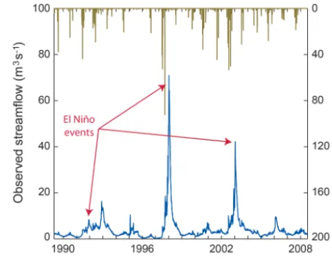
Figure 2. Interannual variability in precipitation and observed streamflow from 1989 to 2008. The hydrological year was defined from May to April so as to capture the snowmelt and peak flow sea-sons at mid-year (the graduations on thexaxis indicate the 1 Jan-uary of each year). Streamflow values are those measured at the catchment outlet before accounting for water abstractions. Precipi-tation values are those obtained after interpolation.

2.3 Hydrological functioning of the catchment 2.3.1 Precipitation variability

during the 1980s and the early 1990s when compared to the late 1990s and the 2000s.

2.3.2 Catchment-scale water balance and dominant processes

Notwithstanding this significant climate variability, a rough estimate of the catchment water balance can be given for the period 2003–2011 using the data presented in the pre-vious subsection and additional information available in the literature. Spatially averaged precipitation ranges from a minimum of 80 mm in 2010 to an estimated maximum of 190 mm in 2008. Evapotranspiration from non-cultivated ar-eas is sufficiently low to be rar-easonably neglected at the basin scale (Kalthoff et al., 2006). By contrast, water losses from the cultivated portions of the basin are likely to be around 10 mm yr−1 _{(Hublart et al., 2014). At high elevations,} sub-limation plays a much greater role than evapotranspiration. Mean annual sublimation rates over two glaciers located in similar, neighbouring catchments have been estimated to be about 1 mm d−1(see, e.g., MacDonell et al., 2013). Thus, a first estimate of the annual water loss associated with snow sublimation can be made by multiplying, for each day of the period, the proportion of the catchment covered with snow by an average rate of 1 mm d−1. This leads to a mean an-nual loss of 70 mm between 2003 and 2011. Note that this value is of the same order of magnitude as those obtained by Favier et al. (2009) using the Weather Research and Forecast-ing regional-scale climate model. Mean annual discharge per unit area varies from a minimum of 20 mm in 2010 to a max-imum of 140 mm in 2003. Interestingly, runoff coefficients exceed 100 % during several years in this period (in 2003, 2006, 2007 and 2009), indicating either an underestimation of precipitation at high elevations, as suggested by Favier et al. (2009), or a delayed contribution of groundwater to sur-face flow from one year to another (Jourde et al., 2011).

Groundwater movement in the catchment is mainly from the mountain blocks toward the valleys and then northward along the riverbed. In the mountains, groundwater flow and storage are controlled primarily by the presence of secondary permeability in the form of joints and fractures (Strauch et al., 2006). The unconfined valley-fill aquifers are replen-ished by mountain front recharge along the valley margins and by infiltration through the channel bed along the losing river reaches (Jourde et al., 2011). Their hydraulic conduc-tivity and saturated thickness range from about 10 m d−1_and 40 m, respectively, in the upper part of the catchment to more than 30 m d−1 _{and 60 m respectively at the outlet} (CAZA-LAC, 2006), allowing a rapid transfer of water to the hy-draulically connected surface streams. Pourrier et al. (2014) studied flow processes and dynamics in the headwaters of the neighbouring Turbio River catchment; yet very little remains currently known about the emergent processes taking place at the catchment scale.

3 Methods

3.1 Multiple-hypothesis modelling framework

In order to evaluate various numerical representations of the catchment functioning, a multiple-hypothesis modelling framework inspired by previous studies in literature was developed. All the models built within this framework are lumped hypotheses run at a daily time step. The modelling process was decomposed into three modules and six model-building decisions. Each module deals with a different as-pect of the precipitation–runoff relationship through one or more decisions (Fig. 3): snow accumulation (A) and melt (B), runoff generation (C), redistribution (D) and delay (E) of wa-ter fluxes, and natural storage effects (F). Each of these deci-sions is provided with a set of alternative modelling options, which are named by concatenating the following elements: first a capital letter from A to F referring to the decision being addressed, then a number from 1 to 3 to distinguish between several competing architectures and, finally, a lower case let-ter froma tocto indicate different parameterizations of the same architecture. Model hypotheses are named by concate-nating the names of the six modelling options used to build them (see Table 4). The models designed within this frame-work share the same overall structure (based on the same series of decisions) but differ in their specific formulations within each decision.

Figure 3. Overall architecture (modules), decision tree and available modelling options of the modular multiple-hypothesis framework (P: catchment-averaged daily precipitation; SWE: snow water equivalent; AE: catchment-averaged daily actual evapotranspiration; S_jj∈[1,5]: state variables of the conceptual stores; Qjj∈[1,5]: water fluxes between the model components).

purpose here is twofold: first, to facilitate the calibration pro-cess by removing any unnepro-cessary (and potentially detrimen-tal) discontinuities from the gradients of the objective func-tions; and second, to provide a more realistic description of hydrological processes across the catchment (Moore, 2007).

3.1.1 Snow accumulation and melt (decisions A and B)

Snow accumulation and melt components deal with the rep-resentation of snow processes at the catchment scale. All modelling options rely on a single conceptual store to ac-cumulate snow during the winter months and release water during the melt season. Decision A refers to the partition-ing of precipitation into rain, snow or a mixture of rain and snow. Decision B refers to the representation of snowmelt processes. Option A1 is the only hypothesis implemented to evaluate the relative abundance of rain and snow. A logis-tic distribution is used in this option instead of usual tem-perature thresholds to implicitly account for spatial varia-tions in rain/snow partitioning over the catchment. In con-trast, three modelling options drawing upon the temperature-index approach (Hock, 2003) are available for the evaluation of snowmelt rates (options B1a, B1b, B1c). Option B1a relies on a constant melt factor while options B1b and B1c allow for temporal variability in the melt factor to reflect seasonal changes in the energy available for melt. A recent example

of option B1c can be found in Clark et al. (2009). Option B1b has been previously applied by Schreider et al. (1997) but at the grid cell scale. Finally, it is worth noting that a smoothing kernel proposed by Kavetski and Kuczera (2007) was introduced in the state equation of the snow reservoir to ignore residual snow remaining in the reservoir outside the snowmelt season.

3.1.2 Runoff generation (decision C)

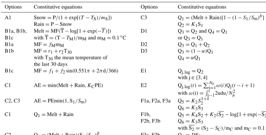
dur-Table 1. Constitutive equations of fluxes between the various components of the modelling options described in Fig. 2. Parameter (in italic) significations and units are detailed in Table 2 (P: catchment-averaged daily precipitation; rain: rain fraction of precipitation P; snow: snow fraction of precipitation P; T: catchment-averaged daily temperature; PE: catchment-averaged daily potential evapotranspiration; AE: catchment-averaged daily actual evapotranspiration; Sj, j∈ [1,5]: state variables of the conceptual stores; Qj, j∈ [1,5]: water fluxes between the model components).

Options Constitutive equations Options Constitutive equations

A1 Snow=P/(1+exp[(T−TS)/mS]) C3 Q1=(Melt+Rain)[1−(1−S1/Sm)b]

Rain=P−Snow Q2=K1S1

B1a, B1b, Melt=MF(T−log[1+exp(−T )]) D1 Q3=Q2and Q4=Q1 B1c with T=(T−TM)/mMand mM=0.1◦C or Q3=Q1

B1a MF=fMmM D2 Q3=Q1+Q2

B1b MF=r1+r2T30 D3 Q3=(1−α)Q1

with T30the mean temperature of Q4=αQ1 the last 30 days

B1c MF=f1+f2sin(0.551π+2πd/366) E1 Qj,lag=Q2 with j∈ {3,4}

C1 AE=min(Melt+Rain, KCPE) E2 Qj,lag(t )=PN_i=b1ω(i)Qj(t−i+1) withω(i)=Ri

i−12udu/Nb2 C2, C3 AE=PEmin(1,S₁/Sm) F1a, F2a, F3a Q₅=K2S21+δ

Q6=K3S3

C1 Q1=Melt+Rain F1b, Q5=K4S2+K2(S2−log[1+exp(−S2)]) F2b, F3b Q6=K3S3

with S2=(S2−SC)/mCand mC=0.1 mm−1 C2 Q1=(Melt+Rain)(S1/Sm)β F3a, F3b Q6=DS2

ing rainfall or snowmelt events, and option C3, in which a leakage from the moisture-accounting store remains possible even after rainfall or snowmelt has ceased. Examples of these two moisture-accounting options can be found in the Hy-drologiska Byråns Vattenbalansavdelning (HBV) (e.g. Seib-ert and Vis, 2012) and probability-distributed model (PDM) (Moore, 2007) rainfall–runoff models. Alternative distribu-tion funcdistribu-tions are available in the literature, for instance in the GR4j (Perrin et al., 2003) and FLEX (Fenicia et al., 2008b) models, but the rationale behind their use remains the same. Actual evapotranspiration is computed from the esti-mated PE using either a constant coefficient (option C1) or a function of the catchment moisture status (options C2 and C3).

3.1.3 Runoff transformation and routing (decisions D to F)

Runoff transformation components account for all the re-tention and translation processes occurring as water moves through the catchment. In practice, junction elements (deci-sion D) and lag functions (deci(deci-sion E) are typically combined with one or more conceptual stores (decision F) to represent the effects of different flow pathways on the runoff process (both timing and volume). Additional elements in the form of lag functions or conceptual stores can also be used to re-flect water routing in the channel network. However, in this study channel routing elements were considered useless at a

daily time step. All the modelling options available for deci-sion F consist of two stores. These can be arranged in parallel (options F1a and F1b), in series (options F2a and F2b), or in a combination of both (options F3a and F3b). In each case, one of the stores has a nonlinear behaviour while the other re-acts linearly. Two types of nonlinear response are provided: one that relies on smoothed thresholds and different storage coefficients (options F1b, F2b and F3b), and the other that re-lies on power laws (options F1a, F2a and F3a). Options F1a and F1b are based on the classical parallel transfer function used in many conceptual models, such as the PDM (Moore, 2007) and the IHACRES (identification of unit hydrographs and component flows from rainfall, evapotranspiration and streamflow) (Jakeman et al., 1993) models, where one store stands for a relatively quick catchment response and the other for a slower response. The structure of options F3a and F3b is very close to the response routine of the HBV model (e.g. Seibert and Vis, 2012). Note that some combinations of mod-elling options were deemed unacceptable and thus not con-sidered (e.g. D3–E1–F1a or D3–E1–F1b).

3.2 Multi-objective optimization 3.2.1 Principle

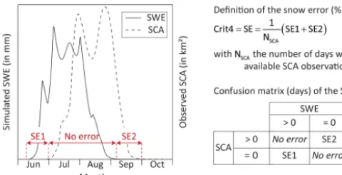
Pareto-Figure 4. Description of the snow error criterion. The overall snow error (SE) can be described as a sum of two terms, SE1 and SE2, whose values are given by a confusion matrix. In this example, wa-ter storage in the snow-accounting store (solid line) starts (SE1) and ends (SE2) sooner than what would be expected from the snow-covered area (SCA) data (dashed line).

optimal solution is achieved when it cannot be improved upon without degrading at least one of its objective criteria. The set of Pareto-optimal solutions for a given model is often called the “Pareto set” and the set of criteria corresponding to this Pareto set is usually referred to as the “Pareto front”. 3.2.2 The NSGA-II algorithm

The Non-dominated Sorted Genetic Algorithm II (NSGA-II) (Deb, 2002) was selected to calibrate the models imple-mented within the multiple-hypothesis framework. This al-gorithm has been used successfully in a number of recent hy-drological studies (see, e.g., Khu and Madsen, 2005; Bekele and Nicklow, 2007; De Vos and Rientjes, 2007; Fenicia et al., 2008a; Shafii and De Smedt, 2009) and has the advantage of not needing any additional parameter (other than those com-mon to all genetic algorithms, i.e. the initial population and the number of generations). Its most distinctive features are the use of a binary tournament selection, a simulated binary crossover and a polynomial mutation operator. For the sake of brevity, the detailed instructions of the algorithm and the conditions of its application to rainfall–runoff modelling can-not be discussed further here. Instead, the reader is referred to the aforementioned literature.

3.2.3 Simulation periods and assessment criteria The simulation period was divided into a rather dry calibra-tion period (1997–2011) and a relatively humid validacalibra-tion period (1982–1996). These two periods were chosen based on data availability to represent contrasted climate condi-tions: the two periods are separated by a shift in the IPO index, as explained in Sect. 2.3.1.

Four criteria were chosen to evaluate the models built within the multiple-hypothesis framework. The first three of them are common to both calibration and validation periods while the fourth criterion differs between the two.

The first criterion is related to the estimation of high flows and draws upon the Nash–Sutcliffe efficiency (NSE) metric:

Crit1=1−NSE= N X

d=1

Qd_obs−Qd_sim 2

N X

d=1

Qd_obs−Qobs 2

(2)

where Qd_obs and Qd_sim are the observed and simulated dis-charges for day d, and N is the number of days with available observations.

The second criterion (NSElog) is related to the estimation of low flows and draws upon a modified, log version of the first criterion:

Crit2=1−NSElog= N X

d=1

log Qd_obs−log Qd_sim 2

N X

d=1

log(Qd_obs)−log Qobs 2

(3)

The third criterion quantifies the mean annual volume error (VEM) made in the estimation of the water balance of the catchment:

Crit3=VEM= Nyears

X

y=1

Vy_obs−Vy_sim/Vy_obsNyears (4)

where Vy_obsand Vy_simare the observed and simulated volumes for year y, and Nyearsis the number of years of the simulation period.

The fourth criterion (Crit4) differs between the two simu-lation periods. In calibration, snow-covered areas (SCA) es-timated from the MODIS data were used to evaluate the con-sistency of snow-accounting modelling options in terms of snow presence or absence at the catchment scale. The ob-jective was to quantify the error made in simulating the sea-sonal dynamics of snow accumulation, storage and melt pro-cesses. Following Parajka and Blöschl (2008), the snow error (SE) was defined as the total number of days when the snow-accounting store of options B1a, B1b and B1c disagreed with the MODIS data as to whether snow was present in the basin (Fig. 4). The number of days with simulation errors is even-tually divided by the total number of days with available MODIS data to express SE as a percentage.

In validation, a cumulated volume error was used to re-place the snow error criterion that could not be computed due to a lack of remotely sensed data over this period:

Crit4=VEC= Nyears X

y=1 Vy_obs−

Nyears X

y=1 Vy_sim

,Nyears X

y=1

3.3 Model selection, model analysis and ensemble modelling

Finally, a total of 72 model structures were implemented and tested within the multi-objective and multiple-hypothesis frameworks. In addition to their names and for purposes of simplicity, these 72 model hypotheses are given a number from 1 to 72 corresponding to their order of appearance in the simulation process (see, e.g., Sect. 4.1).

Model hypotheses can be thought of as points x in the space of performance measures. One possible way to lo-cate these points in space is to consider that each coordi-nate(xi)i=1...4ofxis given by the best performance obtained along the Pareto front of modelxwith respect to theith cri-terion described in Sect. 3.3.2. A clustering technique based on the fuzzy c-means algorithm (Bezdek et al., 1983) and the initialization procedure developed by Chiu (1994) was cho-sen to explore this multi-objective space and identify natural groupings among model hypotheses. To facilitate compar-ison between calibration and validation, the clustering op-erations were repeated independently for each period. The whole experiment, from model-building to multi-objective optimization and cluster identification, was repeated several times to ensure that the final composition of the clusters re-mains the same.

Once the composition of each cluster was established, it was possible to identify a set of “best-performing” clusters for each simulation period, i.e. a set of clusters with the smallest Euclidian distances to the origin of the objective space. The model structures of these “best-performing” clus-ters can be regarded as an equally acceptable representations of the system. An important indicator of structural uncer-tainty is the extent to which the simulation bounds derived from the Pareto sets of these models reproduce the various features of the observed hydrograph. The overall uncertainty envelope should be wide enough to include a large propor-tion of the observed discharge but not so wide that its rep-resentation of the various aspects of the hydrograph (ris-ing limb, peak discharge, fall(ris-ing limb, baseflow) becomes meaningless. In this study, priority was given to maintain-ing at its lowest value the number of outlymaintain-ing observations before searching for the best combination of models which minimized the envelope area. This was achieved iteratively through the following steps:

1. Start with an initial ensemble composed of theNmax models identified as members of the best-performing clusters in both calibration and validation (i.e. models which fail the validation test are ruled out).

2. From now on, consider only the calibration period. Add up the Nmax individual simulation envelopes that can be obtained from the Pareto sets of the Nmax models (hereafter referred to as the “Pareto-envelopes”).

3. Estimate the maximum number of observations enclosed within the resulting overall envelope, Nobs(Nmax), and calculate the area of this envelope, Area(Nmax).

4. Fork=1 toNmax: (a) Identify the

Nmax Nmax−k

possible combinations of Nmaxmodels takenNmax−kat a time.

(b) For each of these combinations,

– add up the individual Pareto-envelopes of the Nmax−k models and calculate the number of observations enclosed within the bounds of the resulting overall envelope,Nobs(Nmax−k); – ifNobs(Nmax−k)=Nobs(Nmax);

– if Area(Nmax−k) < Area (Nmax−k+1) – accept the current combination;

– if Nobs(Nmax−k) < Nobs(Nmax) – reject the current combination.

(c) If all the possible combinations ofNmax−kmodels are rejected, break the loop. The final ensemble of models to consider is the last accepted combination ofNmax−k+1 models.

4 Results

4.1 Model hypotheses evaluation 4.1.1 Cluster analysis

Figure 5. Projections of the clusters onto three possible planes of the objective space in calibration and validation. As explained in Sect. 3.3, each point represents a different model hypothesis.

cluster 1 will be considered as the only best-performing clus-ter. This cluster encompasses 24 members in calibration as against 15 in validation, indicating that several model struc-tures do not pass the validation test (namely model nos. 30, 32, 49, 52, 53, 55, 66, 67, 69 and 72, as shown in Table 4).

Several observations can be made regarding the composi-tion of cluster 1 in both simulacomposi-tion periods. As can be seen from the values listed in Table 4, it is not possible to pick out a single, unambiguous model hypothesis that would per-form better than the others with respect to all criteria. On the one hand, there appears to be several equally acceptable structures for each individual criterion. Model nos. 22 (A1– B1a–C3–D2–E1–F2b), 46 (A1–B1b–C3–D2–E1–F2b) and 54 (A1–B1c–C1–D3–E2–F1b), for instance, yield very simi-lar values of the high-flow criterion (Crit1), despite some dif-ferences in their modelling options. This illustrates the equi-finality of model structures in reproducing one aspect of the system behaviour. On the other hand, some structures seem more appropriate for the simulation of high flows or snow dynamics while others appear to be better at reproducing low flows or estimating the annual water balance of the catch-ment. This indicates trade-offs between model structures in reproducing several aspects of the system behaviour. It is however possible to identify some recurring patterns among the modelling options present in (or absent from) cluster 1 in both periods. First, option B1c is the most represented snowmelt-accounting hypothesis, despite an increase in the number of alternative options (B1a, B1b) in validation. More

strikingly, option C2 is totally absent from cluster 1 in both periods. Single-flux combinations (C1–D1 and C3–D2) and their splitting counterparts (C1–D3 and C3–D1) tend to be equally well represented, thus providing evidence of signifi-cant equifinality among these conceptual representations. Fi-nally, runoff transformation options based on a threshold-like behaviour (F1b, F2b and F3b) account for 75 % of model hy-potheses in calibration and over 90 % in validation. In par-ticular, option F3a turns out to be completely absent from cluster 1 in both periods while models based on option F2a (nos. 49, 55, 67 and 69) fail the validation test. On the oppo-site, option F2b is particularly well represented.

4.1.2 Pareto analysis

Figure 6. Projections of the Pareto fronts of model hypotheses (a) no. 49 (A1-B1c-C1-D1-E1-F2a) and (b) no. 50 (A1-B1c-C1-D1-E1-F2b) onto three possible two-dimensional subspaces of the objective space.

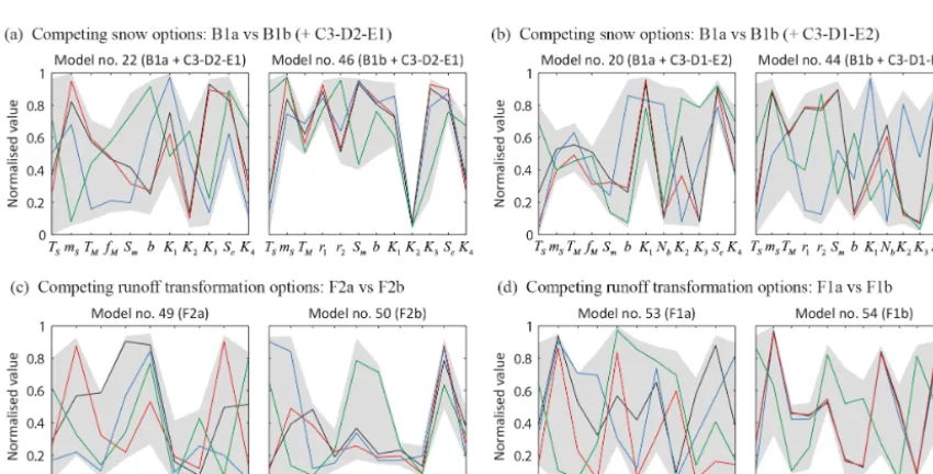
Figure 7. Estimated normalized ranges of the Pareto-optimal sets of eight alternative model structures differing in at least one of their components. The coloured lines stand for the best solutions obtained in calibration with respect to the high-flow criterion (in black), the low-flow criterion (in red), the mean annual volume error (in blue) and the snow error (in green).

(Fig. 6a) than with option F2b (Fig. 6b). This means that op-tion F2a is less efficient in reproducing simultaneously high and low flows and explains why this option disappears from cluster 1 in validation. By contrast, the other pairs of criteria

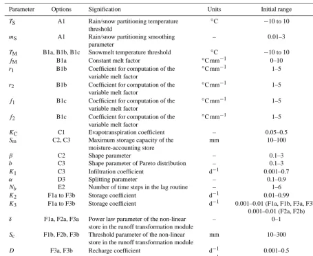
Table 2. Parameters used in the various modelling options with their signification and initial sampling.

Parameter Options Signification Units Initial range

TS A1 Rain/snow partitioning temperature ◦C −10 to 10

threshold

mS A1 Rain/snow partitioning smoothing – 0.01–3

parameter

TM B1a, B1b, B1c Snowmelt temperature threshold ◦C −10 to 10

fM B1a Constant melt factor ◦C mm−1 0–10

r1 B1b Coefficient for computation of the ◦C mm−1 1–5

variable melt factor

r2 B1b Coefficient for computation of the ◦C mm−1 1–5

variable melt factor

f1 B1c Coefficient for computation of the ◦C mm−1 1–5

variable melt factor

f2 B1c Coefficient for computation of the ◦C mm−1 1–5

variable melt factor

KC C1 Evapotranspiration coefficient – 0.05–0.5

Sm C2, C3 Maximum storage capacity of the mm 10–100

moisture-accounting store

β C2 Shape parameter – 0.1–3

b C3 Shape parameter of Pareto distribution – 0.1–3

K1 C3 Infiltration coefficient d−1 0.001–0.7

α D3 Splitting parameter – 0.1–0.9

Nb E2 Number of time steps in the lag routine – 1–6

K2 F1a to F3b Storage coefficient d−1 0.01–0.99

K3 F1a to F3b Storage coefficient d−1 0.001–0.01 (F1a, F1b, F3a, F3b) 0.001–0.01 (F2a, F2b)

δ F1a, F2a, F3a Power law parameter of the non-linear – 0–1

store in the runoff transformation module

Sc F1b, F2b, F3b Threshold parameter of the non-linear mm 10–300 store in the runoff transformation module

D F3a, F3b Recharge coefficient d−1 0.001–0.5

K4 F1b, F2b, F3b Storage coefficient d−1 0.001–0.01

Table 3. Coordinates of the cluster centroids in the four-dimensional (4-D) space of performance measures. The number of models with membership values>50 % (N50 %) is given for each cluster.

Calibration period (1997–2011)

Cluster no. Crit1 (1-NSE) Crit2 (1-NSElog) Crit3 (VEM) (%) Crit4 (SE) (%) N50 %

1 0.15 0.25 10 9 24

2 0.23 0.30 10 10 24

3 0.49 0.58 23 11 10

4 0.60 0.62 25 16 13

5 0.92 0.97 33 20 1

Validation period (1982–1996)

Cluster no. Crit1 (1-NSE) Crit2 (1-NSElog) Crit3 (VEM) (%) Crit4 (VEC) (%) N50 %

1 0.24 0.21 14 3 15

2 0.32 0.29 15 4 25

3 0.38 0.31 15 5 8

4 0.51 0.42 25 23 8

5 0.61 0.44 27 27 11

Table 4. Detailed composition of cluster 1 in calibration and validation. The tables indicate the numbers and the names of the models as well as their number of parameters NP. For each criterion only the best performance value obtained along the Pareto front is given.Npar(%) represents the proportion of observations enclosed within the simulation bounds of each Pareto set of solutions. Asterisks are used to indicate the models which are not in the best-performing group (cluster 1) either in calibration or in validation.

Calibration period (1997–2011)

Model no. Model name (options) NP NSE NSElog VEM(%) SE (%) Npar(%)

2 A1–B1a–C1–D1–E1–F2b 9 0.87 0.76 10.6 11.2 76.0

4 A1–B1a–C1–D1–E1–F3b 10 0.84 0.77 10.4 11.2 53.2

8 A1–B1a–C1–D3–E2–F2b 11 0.83 0.75 11.7 11.1 76.5

20 A1–B1a–C3–D1–E2–F2b 12 0.83 0.76 10.0 11.4 60.0

22 A1–B1a–C3–D2–E1–F2b 11 0.90 0.77 10.4 11.2 64.1

26 A1–B1b–C1–D1–E1–F2b 10 0.87 0.77 10.1 11.5 58.4

30 (*) A1–B1b–C1–D3–E2–F1b 12 0.84 0.70 9.8 11.4 69.6

32 (*) A1–B1b–C1–D3–E2–F2b 12 0.83 0.71 11.1 11.4 68.4

44 A1–B1b–C3–D1–E2–F2b 13 0.89 0.77 10.6 11.4 63.4

46 A1–B1b–C3–D2–E1–F2b 12 0.90 0.76 10.7 11.4 45.4

49 (*) A1–B1c–C1–D1–E1–F2a 9 0.82 0.73 10.9 7.0 67.0

50 A1–B1c–C1–D1–E1–F2b 10 0.86 0.77 10.4 7.0 67.4

52 (*) A1–B1c–C1–D1–E1–F3b 11 0.85 0.72 8.8 8.1 65.7

53 (*) A1–B1c–C1–D3–E2–F1a 11 0.79 0.76 10.8 7.0 63.8

54 A1–B1c–C1–D3–E2–F1b 12 0.90 0.78 11.5 7.5 55.7

55 (*) A1–B1c–C1–D3–E2–F2a 11 0.80 0.73 10.7 7.0 54.5

56 A1–B1c–C1–D3–E2–F2b 12 0.85 0.75 10.8 7.6 76.3

65 A1–B1c–C3–D1–E2–F1a 12 0.83 0.78 8.0 7.7 65.0

66 (*) A1–B1c–C3–D1–E2–F1b 13 0.81 0.77 9.6 6.8 63.5

67 (*) A1–B1c–C3–D1–E2–F2a 12 0.81 0.75 10.7 7.0 73.7

68 A1–B1c–C3–D1–E2–F2b 13 0.85 0.74 10.6 6.8 74.5

69 (*) A1–B1c–C3–D2–E1–F2a 11 0.82 0.73 10.6 7.0 51.8

70 A1–B1c–C3–D2–E1–F2b 12 0.87 0.76 10.7 7.5 76.4

72 (*) A1–B1c–C3–D2–E1–F3b 13 0.81 0.71 9.8 7.1 69.0

Validation period (1982–1996)

Model no. Model name NP NSE NSElog VEM(%) VEC(%) Npar(%)

2 A1–B1a–C1–D1–E1–F2b 9 0.75 0.78 13.3 2.7 87.1

4 A1–B1a–C1–D1–E1–F3b 10 0.73 0.80 14.1 3.8 50.0

8 A1–B1a–C1–D3–E2–F2b 11 0.75 0.76 14.5 5.8 84.8

20 A1–B1a–C3–D1–E2–F2b 12 0.72 0.77 13.7 3.7 58.4

22 A1–B1a–C3–D2–E1–F2b 11 0.76 0.78 12.3 3.3 75.3

26 A1–B1b–C1–D1–E1–F2b 10 0.74 0.78 12.9 3.5 70.2

42 (*) A1–B1b–C3–D1–E2–F1b 13 0.73 0.75 15.6 3.3 62.7

44 A1–B1b–C3–D1–E2–F2b 13 0.74 0.79 13.0 4.1 69.3

46 A1–B1b–C3–D2–E1–F2b 12 0.76 0.77 15.2 3.4 48.4

50 A1–B1c–C1–D1–E1–F2b 10 0.78 0.81 13.9 2.5 73.1

54 A1–B1c–C1–D3–E2–F1b 12 0.77 0.78 15.3 3.5 60.8

56 A1–B1c–C1–D3–E2–F2b 12 0.75 0.77 13.2 4.5 81.3

65 A1–B1c–C3–D1–E2–F1a 12 0.74 0.80 13.8 3.6 73.0

68 A1–B1c–C3–D1–E2–F2b 13 0.77 0.74 13.5 3.7 78.7

70 A1–B1c–C3–D2–E1–F2b 12 0.73 0.78 14.2 3.4 79.4

Further insight into the structural strengths and weak-nesses of model hypotheses can be obtained by determin-ing how parameter values vary along the Pareto fronts of the models. A large “Pareto range” in some parameters indicates structural deficiencies in the corresponding model

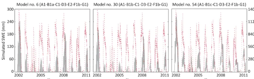
Figure 8. Comparison of MODIS-based SCA data (red dashed lines) with the snow water equivalent (SWE) simulations (shaded areas) of model nos. 6, 30 and 54. The shaded area corresponds to the range of SWE simulations obtained from the Pareto sets of these models.

same pair differ in only one modelling option. Thus, the ef-fects of potential interactions between model constituents are more likely to be detected. Parameter values are normalized using the lower and upper limits given in Table 2 so that all of them lie between 0 and 1. Different colours are used to indi-cate the parameter sets associated with the smallest high-flow (in black), low-flow (in red), volume (in blue) and snow (in green) errors. The extent to which these coloured solutions converge toward the same parameter values or diverge from each other determines the level of parameter identifiability of each model hypothesis. In terms of snow-accounting op-tions, a distinction can be made between snow accumulation paramaters (TSandmS), whose ranges of variation appear to be large in all cases, and snowmelt parameters (TM,fM,r1, r2,f1,f2), whose levels of identifiability depend on interac-tions with the other model components. In Fig. 7a, the Pareto range of snowmelt parameters decreases in width when mov-ing from option B1a to B1b and usmov-ing the combination of options C3–D2–E1. Yet changing this combination into C3– D1–E2 has the opposite effect (Fig. 7b): parameter uncer-tainty now decreases when moving from option B1b to B1a. In terms of runoff transformation parameters (α,Nb,K2,K3, δ,SCandK4), the black and red solutions are closer to each other when options F2b (Fig. 7a, b and c) and F1b (Fig. 7d) are used. By contrast, options F2a (Fig. 7c) and F1a (Fig. 7d) require very different parameter sets to adequately simulate both low and high flows. Again, this suggests that runoff transformation options based on a threshold-like behaviour may be more consistent with the observed data than those based on a power law relationship. It should be noted, how-ever, that relatively large Pareto ranges in some runoff trans-formation parameters (e.g.K2andK3) may still be required to obtain small volume and snow errors at the same time as high low-flow and high-flow performances (e.g. model nos. 44 and 54). Interestingly, the black, red and blue solutions of model nos. 49, 50, 53 and 54 also converge towards the same low values of parameterKC (evapotranspiration coefficient) independently of runoff transformation options.

Drawing any conclusion at this stage about the links between parameter identifiability and model performance might be somewhat hazardous. Other examples (not shown here) show that a model structure may have highly identi-fiable parameter values in calibration and yet not be suited to the conditions prevailing in validation. Also, a reduction of parameter uncertainty as is the case with options F2b and F1b often comes with a greater number of parameters.

Figure 9. Comparison of observed daily discharge at Rivadavia with the overall uncertainty envelope obtained by combining the Pareto-envelopes of eight model structures. These structures have been selected among the 14 members of cluster 1 in both calibration and validation so as to minimize the uncertainty envelope area (Area, in pixels2) while holding constant the number of outlying observations (Outlying, in %). The red parts indicate potential errors in the model structures or observed data.

4.2 Representation of structural uncertainties

This section deals with the identification and use of an en-semble of equally acceptable model structures to quantify and represent the uncertainty arising from the system non-identifiability. Figure 9 shows the overall uncertainty enve-lope obtained with the eight model structures whose com-bination minimizes the envelope area in calibration while holding constant the number of outlying observations (see Sect. 3.3). Over 82 % of discharge observations are captured by the envelope in both simulation periods. Interestingly, this number exceeds the best Npar value obtained in calibration with the individual Pareto-envelopes (see Table 4), which shows how necessary it is to consider an ensemble of model structures. In validation, however, a better combination could be identified since several models of cluster 1 display sig-nificantly higher Npar values (Table 4). On the whole, the comparison of the observed hydrograph with the simulation bounds of the envelope shows a good match of rising limbs and peak discharges in both simulation periods, but a less ac-curate fit of falling limbs during at least one major (in 1987– 1988) and two minor (in 2005–2006 and 2007–2008) events. The slower recession of the observed hydrograph might indi-cate a delayed contribution of one or more catchment com-partments that cannot be described by any of the modelling options available in the multiple-hypothesis framework.

5 Discussion and conclusions

This study aimed at reducing structural uncertainty in the modelling of a semi-arid Andean catchment where lumped conceptual models remain largely under used. To overcome the current lack of information on model adequacy in this catchment, a modular modelling framework (MMF)

rely-ing on six model-buildrely-ing decisions was developed to gen-erate 72 competing model structures. Four assessment crite-ria were then chosen to calibrate and evaluate these models over a 30-year period using the concept of Pareto-optimality. This strategy was designed to characterize both the param-eter uncertainty arising from each model’s structural defi-ciencies (i.e. model inadequacy) and the ambiguity associ-ated with the choice of model components (i.e. model non-uniqueness). Finally, a clustering approach was taken to iden-tify natural groupings in the multi-objective space. Over-all, the greatest source of uncertainty was found in the con-nection between runoff generation and runoff transforma-tion components (decisions D and E). However, the results also showed a significant drop in the number of plausible representations of the system. After validation, 14 model structures among the 24 identified in calibration as the best-performing ones were finally considered as equally accept-able.

so-lutions shown in Fig. 7. Likewise, the frequency of options F2a and F2b in the best-performing cluster suggests that the catchment actually behaves as a “serial” system. The over-all organization of fluxes in the catchment, from high ele-vations toward the valleys and then northward to the out-let, can be conceptualized as a series of two hydraulically connected reservoirs: one standing for the granitic moun-tain blocks (upstream reservoir) and the other for the allu-vial valleys (downstream reservoir). Similar results were also obtained for smaller catchments in Luxembourg character-ized by relatively impervious bedrock and lateral water flows (Fenicia et al., 2014). The results also provided some evi-dence of a strong threshold behaviour at the catchment scale (options F1b, F2b and F3b) compared to the smoother power laws of options F1a, F2a and F3a. However, further research would be needed to track the origin of this behaviour, which might be related at some point to connectivity levels in the fractured and till-mantled areas of the mountain blocks. With regard to snowmelt, the frequent occurrence of option B1c in the best-performing cluster in calibration may indicate a need to account for processes which the degree-day method implemented in option B1a does not fully capture. In semi-arid central Andes (29–30◦S), small zenith angles and a thin, dry and cloud-free atmosphere during most of the year make incoming short-wave radiation the most important source of seasonal variations in the energy available for melt (e.g. Pel-licciotti et al., 2008; Abermann et al., 2013). While this dom-inant source of energy cannot be accounted for by tempera-ture alone, the seasonal timing of snowmelt is also expected to show a greater year-to-year stability, which may explain the relative success of option B1c when compared to option B1b.

Of course, these hypothesized relationships between some physical characteristics of the catchment and specific mod-elling options need to be further qualified. Differentiating between physically adequate and purely numerical solutions will always seem somewhat hazardous in the case of lumped conceptual models. For instance, a small number of models among those identified as the best-performing ones also rely on parallel (F1a, F1b) and intermediate (F3b) runoff transfor-mation options. Also, the relative proportions of snowmelt-accounting options B1a, B1b and B1c, appears much more balanced in validation, where no snow error criterion could be applied, than in calibration. Although this was not our ob-jective in this paper, comparative studies including several similar or contrasted catchments would be required to better understand how different model structures relate to different physical settings. Such understanding is of primary impor-tance to the choice of conceptual models in climate change impact studies.

5.2 Model parsimony

Another important issue related to model identification is the extent to which the “principle of parsimony” can be applied

to differentiate between a large number of model hypotheses. Many authors rightly consider that a maximum of 5 to 6 pa-rameters should be accepted in calibration when using a sin-gle objective function. Efstratiadis and Koutsoyiannis (2010) extended this empirical rule to the case of multi-objective schemes by allowing “a ratio of about 1:5 to 1:6 between the number of criteria and the number of parameters to op-timize”. For a multi-objective scheme based on four crite-ria (as in the present study), this leads to consider 20 to 24-parameter models as still being parsimonious. This will certainly seem unreasonable to many modelers because, as Efstratiadis and Koutsoyiannis (2010) also pointed out, the various criteria used are generally not independent of each other. In our case, for instance, the information added by the low-flow criterion may not be so different from that al-ready introduced by the high-flow criterion. By contrast, the snow criterion tends to add new information on the snow-related parameters. From this perspective, it is noteworthy that most rejected hypotheses among the 24 identified in cal-ibration as members of cluster 1 had more than 11 free pa-rameters, with only one having 9 parameters. The principle of parsimony, however, cannot be used to further discrimi-nate between the remaining 14 best-performing hypotheses. For instance, model no. 54 (12 parameters) performs better than model no. 2 (9 parameters) with respect to the high-flow criterion.

5.3 Uncertainty quantification

Eventually, the number of models used to represent struc-tural uncertainty was reduced by searching for which min-imal set of models maximized the number of observations covered by the ensemble of Pareto-envelopes. It is impor-tant to make clear that model inadequacy and non-uniqueness were evaluated here in non-probabilistic terms. In particular, the Pareto-envelopes derived for each model structure quan-tify only the uncertainty arising from the trade-offs between competing criteria and do not have a predefined statistical meaning (Engeland et al., 2006). Consequently, the overall simulation bounds shown in Fig. 9 cannot be easily inter-preted as “confidence bands”. Although discussing the ad-equacy of non-probabilistic approaches to structural uncer-tainty was far beyond the scope of this study, it is interesting to analyze the reasons why between 15 and 20 % of the ob-servations remained outside the overall simulated envelope in both calibration and validation. To a large extent, this lack of performance can be attributed either to an insufficient cover-age of the hypothesis and objective spaces or to uncertainties in the precipitation and streamflow data that were overlooked in this study.

in-put errors (e.g. Freer et al., 2003; Beven, 2006). Also, this concept should not be confused with that of equifinality. Both notions agree that it is not possible to identify a sin-gle, best solution to the calibration problem and that multi-ple parameters sets should be retained to give a proper ac-count of model uncertainty. However, the Pareto set of so-lutions represents the minimum parameter uncertainty that can be achieved when several criteria are considered simul-taneously with no a priori preference for one over the others (Gupta et al., 2003). By contrast, two parameter sets are said to be equifinal (in a statistical sense) if they can be regarded as equally acceptable with respect to a given model outcome. For a proper assessment of parameter equifinality, more prob-abilistic approaches should be taken (Madsen, 2000; Huis-man et al., 2010). In the context of multiple-hypothesis test-ing, a meticulous selection of the assessment criteria is also critical to avoid rejecting some modelling options for the wrong reasons. For instance, the snow error criterion was shown to have a great influence on the identification of snow-accounting components, as much more ambiguity between the various available options was observed during the valida-tion period when this criterion could not be used. Also, like any other multiple-hypothesis framework, the MMF devel-oped in this study suffers from an insufficient coverage of the hypothesis space (Gupta et al., 2012). The parameterization of evapotranspiration, for example, was not considered as an independent model-building decision. Only one formula was applied to calculate potential evapotranspiration and the possibility to retrieve actual evapotranspiration from down-stream water stores was not provided. Likewise, the runoff transformation process was described using only two water stores, of which only one was assumed to have a nonlinear behaviour. Future work to improve the conceptual modelling of the Claro River catchment should include the testing of new or refined hypotheses to allow for the use of additional auxiliary data (e.g. observed snow heights or irrigation water use).

5.4 Data quality issues

More fundamentally, our ability to discriminate among the competing model hypotheses was constrained by inevitable errors in the input and output data sets. In particular, the com-parison of simulated SWE levels and MODIS-based SCA es-timates revealed some uncertainty in the estimation of pre-cipitation inputs and confirmed previous results obtained by Favier et al. (2009). Some precipitation events occurring in the early winter may not be captured by the gauging net-work (<3200 m a.s.l.) used for the interpolation of precip-itation across the catchment. These errors may add to sys-tematic volume errors caused by wind, wetting and evapo-ration losses at the gauge level, leading to an overall under-estimation of precipitation, as indicated by the rough esti-mate of the catchment-scale water balance given in Sect. 2. It was also possible to highlight some errors in the streamflow

data. The observed streamflow was “naturalized” by sim-ply adding back the estimated historical water abstractions (Sect. 2.2). When applied on a daily basis, this process in-evitably adds some uncertainty to streamflow values because a significant part of surface-water abstractions actually re-turn to the river system within a few days due to conveyance and field losses. In general, ignoring these return flows would lead to overestimating daily natural flows. In this paper, how-ever, the actual water withdrawals were not known with pre-cision but only as percentages of the nominal water rights – these percentages being fixed on a monthly basis by the au-thorities to account for variations in water availability. The combined impact of streamflow and precipitation errors on the assessment of structural uncertainty thus remained un-known. Further research is currently underway to integrate the effects of water abstractions and crop water use in the hy-drological modelling process (Hublart et al., 2015; see also Kiptala et al., 2014 for another approach). From a multiple-hypothesis perspective, the modelling of irrigation water use should be regarded as a testable model component in its own right.

Acknowledgements. The authors are very grateful to the Centro de

Estudios Avanzados en Zonas Áridas (CEAZA) for its essential logistic support during the field missions and to Gustavo Freixas from the Dirección General de Agua (Chile) for providing the necessary streamflow data. The authors also thank S. Lhermitte, D. López and S. MacDonell for providing the MODIS data used in this study and S. Gascoin for informal advice and much useful dis-cussion. Moreover, the authors thank the two anonymous reviewers for their interest in this work and for their useful comments that helped to improve the article.

Edited by: T. Kjeldsen

References

Abermann, J., Kinnard, C., and MacDonell, S.: Albedo variations and the impact of clouds on glaciers in the Chilean semi-arid Andes, J. Glaciol., 60, 183–191, 2013.

Bekele, E. G. and Nicklow, J. W.: Multi-objective automatic calibra-tion of SWAT using NSGA-II, J. Hydrol., 341, 165–176, 2007. Beven, K.: Prophecy, reality and uncertainty in distributed

hydro-logical modelling, Adv. Water Resour., 16, 41–51, 1993. Beven, K.: A Manifesto for the Equifinality Thesis, J. Hydrol., 320,

18–36, 2006.

Bezdek, J. C., Ehrlich, R., and Full, W.: FCM: The fuzzy c-means clustering algorithm, Comput. Geosci., 10, 191–203, 1983. Birkel, C., Tetzlaff, D., Dunn, S. M., and Soulsby, C.: Towards

a simple dynamic process conceptualization in rainfall–runoff models using multi-criteria calibration and tracers in temper-ate, upland catchments, Hydrol. Process., 24, 260–275, 2010. Blöschl, G. and A. Montanari: Climate change impacts–throwing the dice?, Hydrol. Process., 24, 374–381, 2010.

Boyle, D. P., Gupta, H. V., and Sorooshian, S.: Toward improved calibration of hydrologic models: Combining the strengths of manual and automatic methods, Water Resour. Res., 36, 3663– 3674, 2000.

Buytaert, W. and K. Beven: Models as multiple working hypothe-ses: hydrological simulation of tropical alpine wetlands, Hydrol. Process., 25, 1784–1799, 2011.

Capell, R., Tetzlaff, D., and Soulsby, C.: Can time domain and source area tracers reduce uncertainty in rainfall-runoff models in larger heterogeneous catchments?, Water Resour. Res., 48, W09544, doi:10.1029/2011WR011543, 2012.

Caviedes, C. N. and Paskoff, R.: Quaternary glaciations in the An-des of north-central Chile, J. Glaciol., 14, 155–169, 1975. Centro del Agua para Zonas Áridas y semiáridas de América Latina

y el Caribe (CAZALAC): Aplicación de metodologías para de-terminar la eficiencia de uso del agua – Estudio de caso en la Región de Coquimbo. Informe Técnico, Gobierno Regional, Santiago (Chile), 2006.

Chiu, S.: Fuzzy model identification based on cluster estimation, J. Intell. Fuzzy Syst., 2, 267–278, 1994.

Clark, M. P., Slater, A. G., Barrett, A. P., Hay, L. E., McCabe, G. J., Rajagopalan, B., and Leavesley, G. H.: Assimilation of snow covered area information into hydrologic and landsurface mod-els, Adv. Water Resour., 29, 1209–1221, 2006.

Clark, M. P., Slater, A. G., Rupp, D. E., Woods, R. A., Vrugt, J. A., Gupta, H. V., Wagener, T., and Hay, L. E.: Framework for Understanding Structural Errors (FUSE): A modular framework to diagnose differences between hydrological models, Water Re-sour. Res., 44, W00B02, doi:10.1029/2007WR006735, 2008. Clark, M., Hreinsson, E. O., Martinez, G., Tait, A., Slater, A.,

Hen-drikx, J., Owens, I., Gupta, H., Schmidt, J., and Woods, R.: Sim-ulations of seasonal snow for the South Island, New Zealand, J. Hydrol., 48, 41–58, 2009.

Clark, M. P., Kavetski, D., and Fenicia, F.: Pursuing the method of multiple working hypotheses for hydrological modelling, Water Resour. Res., 47, W09301, doi:10.1029/2010WR009827, 2011. Collet, L., Ruelland, D., Borrell-Estupina, V., Dezetter, A., and

Ser-vat, E.: Integrated modelling to assess long-term water supply ca-pacity of a meso-scale Mediterranean catchment, Sci. Total Env-iron., 461/462, 528–540, 2013.

Coxon, G., Freer, J., Wagener, T., Odoni, N. A., and Clark, M. P.: Diagnostic evaluation of multiple hypotheses of hy-drological behaviour in a limits-of-acceptability framework for 24 UK catchments, Hydrol. Process., 28, 6135–6150, doi:10.1002/hyp.10096, 2013.

De Vos, N. J. and Rientjes, T. H. M.: Multi-objective performance comparison of an artificial neural network and a conceptual rainfall-runoff model, Hydrolog. Sci. J., 52, 397–413, 2007. Deb, K., Pratap. A, Agarwal, S., and Meyarivan, T.: A fast and

eli-tist multiobjective genetic algorithm: NSGA-II, IEEE T. Evolut. Comput., 6, 181–197, 2002.

Dooge, J.: Looking for hydrologic laws, Water Resour. Res., 22, 46S–58S, doi:10.1029/WR022i09Sp0046S, 1986.

Dooge, J.: Searching for Simplicity in Hydrology, Surv. Geophys., 18, 511–534, 1997.

Efstratiadis, A. and Koutsoyiannis, D.: One decade of multi-objective calibration approaches in hydrological modelling: a re-view, Hydrolog. Sci. J., 55, 58–78, 2010.

Ehret, U., Gupta, H. V., Sivapalan, M., Weijs, S. V., Schymanski, S. J., Blöschl, G., Gelfan, A. N., Harman, C., Kleidon, A., Bogaard, T. A., Wang, D., Wagener, T., Scherer, U., Zehe, E., Bierkens, M. F. P., Di Baldassarre, G., Parajka, J., van Beek, L. P. H., van Griensven, A., Westhoff, M. C., and Winsemius, H. C.: Advanc-ing catchment hydrology to deal with predictions under change, Hydrol. Earth Syst. Sci., 18, 649–671, doi:10.5194/hess-18-649-2014, 2014.

Engeland, K., Braud, I., Gottschalk, L., and Leblois, E.: Multi-objective regional modelling, J. Hydrol., 327, 339–351, 2006. Favier, V., Falvey, M., Rabatel, A., Praderio, E., and López, D.:

Interpreting discrepancies between discharge and precipitation in high-altitude area of Chile’s Norte Chico region (26–32◦S), Water Resour. Res., 45, W02424, doi:10.1029/2008WR006802, 2009.

Fenicia, F., McDonnell, J. J., and Savenije, H. H. G.: Learning from model improvement: On the contribution of complementary data to process understanding, Water Resour. Res., 44, W06419, doi:10.1029/2007WR006386, 2008a.

Fenicia, F., Savenije, H. H. G., Matgen, P., and Pfister, L.: Understanding catchment behavior through stepwise model concept improvement, Water Resour. Res., 44, W01402, doi:10.1029/2006WR005563, 2008b.

Fenicia, F., Kavetski, D., and Savenije, H. H. G.: Elements of a flexible approach for conceptual hydrological modelling: 1. Mo-tivation and theoretical development, Water Resour. Res., 47, W11510, doi:10.1029/2010WR010174, 2011.

Fenicia, F., Kavetski, D., Savenije, H. H. G., Clark, M. P., Schoups, G., Pfister, L., and Freer, J.: Catchment properties, function, and conceptual model representation: is there a correspondence?, Hy-drol. Process., 28, 2451–2467, 2014.

Freer, J., Beven, K., and Peters, N.: Multivariate Seasonal Pe-riod Model Rejection Within the Generalised Likelihood Uncer-tainty Estimation Procedure, in Calibration of Watershed Mod-els, edited by: Duan, Q., Gupta, H. V., Sorooshian, S., Rousseau, A. N., and Turcotte, R., Am. Geophys. Union, Washington, DC, 69–87, 2003.

Gupta, H. V., Sorooshian, S., and Yapo, P. O.: Toward improved cal-ibration of hydrologic models: Multiple and noncommensurable measures of information, Water Resour. Res., 34, 751–763, 1998. Gupta, H. V., Bastidas, L. A., Vrugt, J. A., and Sorooshian, S.: Mul-tiple criteria global optimization for watershed model calibration, Water Sci. Appl., 6, 125–132, 2003.

Gupta, H. V., Clark, M. P., Vrugt, J. A., Abramowitz, G., and Ye, M.: Towards a comprehensive assessment of model structural adequacy, Water Resour. Res., 48, W08301, doi:10.1029/2011WR011044, 2012.

Hock, R.: Temperature index melt modelling in mountain areas, J. Hydrol., 282, 104–115, 2003.

Hublart, P., Ruelland, D., Dezetter, A., and Jourde, H.: Mod-elling current and future trends in water availability for agri-culture on a semi-arid and mountainous Chilean catchment, in: Cold and Mountain Region Hydrological Systems Under Cli-mate Change: Towards Improved Projections, IAHS-AISH P., 360, 26–32, 2013.

7th FRIEND Int. Conf., Montpellier, France, 24–28 February 2014, IAHS-AISH P., 363, 209–214, 2014.

Hublart, P., Ruelland, D., García de Cortázar Atauri, I., and Iba-cache, A.: Assessing the reliability of conceptual hydrologi-cal modelling in a cultivated, drought-prone catchment of the Chilean Andes, in: Hydrologic Non-Stationarity and Extrapolat-ing Models to Predict the Future, IAHS-AISH P, 92, 1–7, 2015. Huisman, J. A., Rings, J., Vrugt, J. A., Sorg, J., Vereecken, H.:

Hy-draulic properties of a model dike from coupled Bayesian and multi-criteria hydrogeophysical inversion, J. Hydrol., 380, 62– 73, 2010.

IPCC: Full Report: the Physical Science Basis, in: Contribution of Working Group I to the Fifth Assessment Report of the Inter-governmental Panel on Climate Change, Climate Change 2013, edited by: Stocker, T. F., Qin, D., Plattner, G.-K., Tignor, M., Allen, S. K., Boschung, J., Nauels, A., Xia, Y., Bex, V., and Midgley, P. M., Cambridge University Press, Cambridge, UK and New York, NY, USA, 1261–1264, 2013.

Jakeman, A. J. and Hornberger, G. M.: How much complexity is warranted in a rainfall-runoff model?, Water Resour. Res., 29, 2637–2649, 1993.

Jakeman, A. J. and Letcher, R. A.: Integrated assessment and mod-elling: features, principles and examples for catchment manage-ment, Environ. Modell. Softw., 18, 491–501, 2003.

Jothityangkoon, C., Sivapalan, M., and Farmer, D. L.: Process con-trols of water balance variability in a large semi-arid catchment: downward approach to hydrological model development, J. Hy-drol., 254, 174–198, 2001.

Jourde, H., Rochette, R., Blanc, M., Brisset, N., Ruelland, D., Freixas, G., and Oyarzun, R. : Relative contribution of ground-water and surface ground-water fluxes in response to climate variability of a mountainous catchment in the Chilean Andes, in: Cold Re-gions Hydrology in a Changing Climate, IAHS-AISH P., 346, 180–188, 2011.

Kalthoff, N., Fiebig-Wittmaack, M., Meißner, C., Kohler, M., Uri-arte, M., Bischoff-Gauß, I., and Gonzales, E.: The energy bal-ance, evapo-transpiration and nocturnal dew deposition of an arid valley in the Andes, J. Arid Environ., 65, 420–443, 2006. Kavetski, D. and Fenicia, F.: Elements of a flexible

ap-proach for conceptual hydrological modelling: 2. Application and experimental insights, Water Resour. Res., 47, W11511, doi:10.1029/2011WR010748, 2011.

Kavetski, D. and Kuczera, G.: Model smoothing strategies to re-move microscale discontinuities and spurious secondary optima in objective functions in hydrological calibration, Water Resour. Res., 43, W03411, doi:10.1029/2006WR005195, 2007. Khu, S. T., and Madsen, H.: Multiobjective calibration with

Pareto preference ordering: An application to rainfall-runoff model calibration, Water Resour. Res., 41, W03004, doi:10.1029/2004WR003041, 2005.

Kiptala, J. K., Mul, M. L., Mohamed, Y. A. and van der Zaag, P.: Modelling stream flow and quantifying blue water using a mod-ified STREAM model for a heterogeneous, highly utilized and data-scarce river basin in Africa, Hydrol. Earth Syst. Sci., 18, 2287–2303, 2014,

http://www.hydrol-earth-syst-sci.net/18/2287/2014/.

Kirchner, J. W.: Getting the right answers for the right rea-sons: Linking measurements, analyses, and models to advance

the science of hydrology, Water Resour. Res., 42, WR004362, doi:10.1029/2005WR004362, 2006.

Kokkonen, T. S. and Jakeman, A. J.: A comparison of metric and conceptual approaches in rainfall-runoff modelling and its impli-cations, Water Resour. Res., 37, 2345–2352, 2001.

Krueger, T., Freer, J., Quinton, J. N., Macleod, C. J. A., Bilotta, G. S., Brazier, R. E., Butler, P., and Haygarth, P. M.: Ensemble eval-uation of hydrological model hypotheses, Water Resour. Res., 46, W07516, doi:10.1029/2009WR007845, 2010.

Lee, G., Tachikawa, Y., and Takara, K.: Comparison of model struc-tural uncertainty using a multi-objective optimization method, Hydrol. Process., 25, 2642–2653, 2011.

MacDonell, S., Kinnard, C., Mölg, T., Nicholson, L., and Aber-mann, J.: Meteorological drivers of ablation processes on a cold glacier in the semiarid Andes of Chile, The Cryosphere, 7, 1833– 1870, doi:10.5194/tc-7-1513-2013, 2013.

Madsen, H.: Automatic calibration of a conceptual rainfall–runoff model using multiple objectives, J. Hydrol., 235, 276–288, 2000. McDonnell, J. J., Sivapalan, M., Vaché, K., Dunn, S., Grant, G., Haggerty, R., Hinz, C., Hooper, R., Kirchner, J., Roderick, M. L., Selker, J., and Weiler, M.: Moving beyond heterogeneity and pro-cess complexity: A new vision for watershed hydrology, Water Resour. Res., 43, W07301, doi:10.1029/2006WR005467, 2007. McMillan, H.: Effect of spatial variability and seasonality in soil

moisture on drainage thresholds and fluxes in a conceptual hy-drological model, Hydrol. Process., 26, 2838–2844, 2012a. McMillan, H., Tetzlaff, D., Clark, M., and Soulsby, C.: Do

time-variable tracers aid the evaluation of hydrological model struc-ture? A multimodel approach, Water Resour. Res., 48, W05501, doi:10.1029/2011WR011688, 2012b.

Michaud, J. and Sorooshian, S.: Comparison of simple versus com-plex distributed runoff models on a semi-arid watershed, Water Resour. Res., 30, 593–605, 1994.

Milano, M., Ruelland, D., Dezetter, A., Fabre, J., Ardoin-Bardin, S., and Servat, E.: Modelling the current and future capacity of water resources to meet water demands in the Ebro basin, J. Hydrol., 500, 114–126, 2013.

Minville, M., Brissette, F., and Leconte, R.: Uncertainty of the im-pact of climate change on the hydrology of a nordic watershed, J. Hydrol., 358, 70–83, 2008.

Montecinos, A. and Aceituno, P.: Seasonality of the ENSO-Related Rainfall Variability in Central Chile and Associated Circulation Anomalies, J. Climate, 16, 281–296, 2003.

Moore, R. J.: The PDM rainfall-runoff model, Hydrol. Earth Syst. Sci., 11, 483–499, doi:10.5194/hess-11-483-2007, 2007. Oudin, L., Hervieu, F., Michel, C., Perrin, C., Andréassian, V.,

Anc-til, F., and Loumagne, C.: Which potential evapotranspiration in-put for a lumped rainfall–runoff model?: Part 2—Towards a sim-ple and efficient potential evapotranspiration model for rainfall– runoff modelling, J. Hydrol., 303, 290–306, 2005.

Parajka, J. and Blöschl, G.: The value of MODIS snow cover data in validating and calibrating conceptual hydrologic models, J. Hy-drol., 358, 240–258, 2008.