A new probability density function for spatial distribution of soil water storage capacity leads to the SCS curve number method

https://doi.org/10.5194/hess-22-6567-2018 © Author(s) 2018. This work is distributed under the Creative Commons Attribution 4.0 License.

A new probability density function for spatial distribution of soil

water storage capacity leads to the SCS curve number method

Dingbao Wang

Department of Civil, Environmental, and Construction Engineering, University of Central Florida, Orlando, Florida, USA Correspondence:Dingbao Wang ([email protected])

Received: 24 January 2018 – Discussion started: 13 February 2018

Revised: 29 October 2018 – Accepted: 9 December 2018 – Published: 20 December 2018

Abstract. Following the Budyko framework, the soil wet-ting ratio (the ratio between soil wetwet-ting and precipitation) as a function of the soil storage index (the ratio between soil wetting capacity and precipitation) is derived from the Soil Conservation Service Curve Number (SCS-CN) method and the variable infiltration capacity (VIC) type of model. For the SCS-CN method, the soil wetting ratio approaches 1 when the soil storage index approaches∞, due to the limitation of the SCS-CN method in which the initial soil moisture condi-tion is not explicitly represented. However, for the VIC type of model, the soil wetting ratio equals the soil storage in-dex when the soil storage inin-dex is lower than a certain value, due to the finite upper bound of the generalized Pareto dis-tribution function of storage capacity. In this paper, a new distribution function, supported on a semi-infinite interval x∈ [0,∞), is proposed for describing the spatial distribu-tion of storage capacity. From this new distribudistribu-tion funcdistribu-tion, an equation is derived for the relationship between the soil wetting ratio and the storage index. In the derived equation, the soil wetting ratio approaches 0 as the storage index ap-proaches 0; when the storage index tends to infinity, the soil wetting ratio approaches a certain value (≤1) depending on the initial storage. Moreover, the derived equation leads to the exact SCS-CN method when initial water storage is 0. Therefore, the new distribution function for soil water stor-age capacity explains the SCS-CN method as a saturation ex-cess runoff model and unifies the surface runoff modeling of the SCS-CN method and the VIC type of model.

1 Introduction

The Soil Conservation Service Curve Number (SCS-CN) method (Mockus, 1972) has been popularly used for direct runoff estimation in engineering communities. Even though the SCS-CN method was obtained empirically (Ponce, 1996; Beven, 2012), it is often interpreted as an infiltration ex-cess runoff model (Bras, 1990; Mishra and Singh, 1999). Yu (1998) showed that partial area infiltration excess runoff generation on a statistical distribution of soil infiltration char-acteristics provided a similar runoff generation equation to the SCS-CN method. Recently, Hooshyar and Wang (2016) derived an analytical solution for Richards’ equation for ponded infiltration into a soil column bounded by a water table, and they showed that the SCS-CN method, as an in-filtration excess model, is a special case of the derived gen-eral solution. The SCS-CN method has also been interpreted as a saturation excess runoff model (Steenhuis et al., 1995; Lyon et al., 2004; Easton et al., 2008). During an interview, Mockus, who developed the proportionality relationship of the SCS-CN method, stated that “saturation overland flow was the most likely runoff mechanism to be simulated by the method” (Ponce, 1996). Recently, Bartlett et al. (2016a) developed a probabilistic framework, which provides a sta-tistical justification of the SCS-CN method and extends the saturation excess interpretation of the event-based runoff of the method.

variability of soil moisture storage capacity is described by a cumulative probability distribution function in the Xinan-jiang model (Zhao, 1977; Zhao et al., 1992) and the vari-able infiltration capacity (VIC) model (Wood et al., 1992; Liang et al., 1994). The spatial distribution of storage capac-ity in these models is described by the generalized Pareto distribution, which has been used for catchment-scale runoff prediction and large-scale land surface hydrologic simula-tions. Bartlett et al. (2016b) proposed an event-based prob-abilistic storage framework for unifying TOPMODEL, the VIC type of model, and the SCS-CN method, and the frame-work includes a spatial description of the runoff concept of “prethreshold” and “threshold-excess” runoff (Bartlett et al., 2016a).

Even though the SCS-CN method has been interpreted as a saturation excess runoff model in the literature, there is a knowledge gap for the direct linkage between the SCS-CN method and the Xinanjiang and VIC type of model based on a probability distribution function for the spatial variability of soil water storage capacity. If the SCS-CN method is a saturation excess runoff model, is there a distribution func-tion for soil water storage capacity which leads to the SCS-CN method? If yes, what is the probability density function (PDF)? This is an unsolved research question. The objective of this paper is to fill this knowledge gap, i.e., discovering the distribution function for soil water storage capacity which leads to the SCS-CN method. This is a procedure of inverse modeling, i.e., identifying the distribution function of the sat-uration excess runoff model for a known functional form of runoff generation.

Meanwhile, the identification of the new distribution function is intrigued by the linkage between the SCS-CN method and the Budyko equation (Budyko, 1974). By ap-plying the generalized proportionality hypothesis from the SCS-CN method to mean annual water balance, Wang and Tang (2014) derived a one-parameter Budyko equation for the mean annual evaporation ratio (i.e., the ratio of evapora-tion to precipitaevapora-tion) as a funcevapora-tion of the climate aridity index (i.e., the ratio of potential evaporation to precipitation). As an analogy to the Budyko framework, the SCS-CN method and the VIC type of model at the event scale can be represented by the relationship between the soil wetting ratio, defined as the ratio between soil wetting and precipitation, and the soil storage index, which is defined as the ratio between soil wet-ting capacity and precipitation. The representation of runoff generation in the Budyko type of framework facilitates the identification of the new distribution function for soil water storage capacity leading to the SCS-CN method.

The identified new distribution function for soil water stor-age capacity will unify the SCS-CN method and the VIC type of model. In Sect. 2, the SCS-CN method is presented in the form of the Budyko-type framework with two parameteri-zation schemes. In Sect. 3, the VIC type of model is pre-sented in the form of the Budyko-type framework. In Sect. 4, the SCS-CN method is then compared with the VIC type of

model from the perspectives of the number of parameters and boundary conditions (i.e., the lower and upper bounds of the soil storage index). In Sect. 5, the proposed new distribution function is introduced and compared with the generalized Pareto distribution of the VIC type of model, and a modi-fied SCS-CN method considering initial storage explicitly is derived from the new distribution function. Conclusions are drawn in Sect. 6.

2 SCS curve number method

In this section, the SCS-CN method is described in the form of surface runoff modeling and then is presented for infil-tration modeling in the Budyko-type framework. The initial storage at the beginning of a time interval (e.g., rainfall event) is denoted byS0(mm), and the maximum value of average

storage capacity over the catchment is denoted bySb(mm).

The storage capacity for soil wetting for the time interval, Sp(mm), is computed by

Sp=Sb−S0. (1)

The total rainfall during the time interval is denoted byP (mm). Before surface runoff is generated, a portion of rainfall is intercepted by vegetation and infiltrates into the soil. This portion of rainfall is called initial abstraction or initial soil wetting denoted byWi(mm). The remaining rainfall (P−Wi)

is partitioned into runoff and continuing soil wetting. This competition is captured by the proportionality relationship in the SCS-CN method:

W−Wi

Sp−Wi

= Q

P−Wi

, (2)

whereW(mm) is the total soil wetting,W−Wiis continuing

wetting andSp−Wiis its potential value,Q(mm) is surface

runoff, andP−Wi is the available water and interpreted as

the potential value ofQ. Since rainfall is partitioned into to-tal soil wetting and surface runoff, i.e.,P =W+Q, surface runoff is computed by substitutingW=P−Qinto Eq. (2):

Q= (P−Wi)

2

P +Sp−2Wi

. (3)

This equation is used for computing direct runoff in the SCS-CN method.

The SCS-CN method can also be represented in terms of the soil wetting ratio W_P. Substituting Eq. (3) into W= P−Qand dividingP on both sides, the soil wetting ratio equation is obtained:

W P =

Sp

P − W2

i

P2

1+Sp

P −2 Wi

P

. (4)

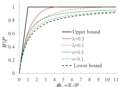
Figure 1.The wetting ratioW_Pversus the soil storage indexS_Pp from the SCS-CN method based on two parameterization schemes:

λ= Wi

Sp−Wi (scheme 1) andε=

Wi

W (scheme 2).

index, both available water supply and water demand are de-termined by climate.

8sc=

Sp

P (5)

A similar dimensionless parameter for the ratio between the maximum soil storage capacity and mean rainfall depth of rainfall events was defined in Porporato et al. (2004). In the soil storage index, water demand is determined by soil and available water supply is determined by climate. Substituting Eq. (5) into Eq. (4), the soil wetting equation for the SCS-CN method is obtained:

W P =

8sc− W2

i

P2

1+8sc−2W_Pi

. (6)

There are two potential schemes for parameterizing the initial wetting in Eq. (6). As the first scheme, the initial wetting is usually parameterized as the ratio between initial wetting and storage capacity in the SCS-CN method. The detail of this scheme is described in Appendix A and plotted in Fig. 1. As we can see, the range of8scis dependent on the parameter

λ= Wi

Sp−Wi.

In order to avoid the situation where the range of 8sc is

dependent on the parameterλ, we can use the following pa-rameterization scheme (Chen et al., 2013; Tang and Wang, 2017):

ε=Wi

W. (7)

Substituting Eq. (7) into Eq. (6), we can obtain the following equation:

W P =

1+8sc−

p

(1+8sc)2−4ε (2−ε) 8sc

2ε (2−ε) . (8)

Equation (8) has the same functional form as the derived Budyko equation for the long-term evaporation ratio (Wang

and Tang, 2014; Wang et al., 2015). Equation (8) satisfies the following boundary conditions: W_P →0 as8sc→0 and W

P →1 as8sc→ ∞. Based on Eq. (7), the range of ε is

[0,1], and ε=1 corresponds to the upper bound (Fig. 1). Equation (8) becomes Eq. (A3) asε→0, and it is the lower bound. Figure 1 plots Eq. (8) forε=0.1 and 0.3. Due to the dependence of the range of8sc on the parameter λ in the

first parameterization scheme, the second parameterization scheme is focused on in the following sections.

In the SCS-CN method, the soil wetting ratio is a function of the soil storage index with a parameter for describing ini-tial wetting. The average wetting capacity at the catchment scale is used for computing the soil storage index, but the spatial variability of wetting capacity is not represented in the SCS-CN method.

3 Saturation excess runoff model

The spatial variability of soil water storage capacity is explic-itly represented in the saturation excess runoff models such as VIC and Xinanjiang. In these models, the spatial variation of the point-scale storage capacity (C) is represented by a generalized Pareto distribution:

F (C)=1−

1− C Cm

β

, (9)

whereF (C)is the cumulative probability, i.e., the fraction of the catchment area for which the storage capacity is less than C (mm), andCm(mm) is the maximum value of the

point-scale storage capacity over the catchment. The water storage capacity includes vegetation interception, surface retention, and soil moisture capacity;β is the shape parameter of the storage capacity distribution and is usually assumed to be a positive number.β ranges from 0.01 to 5.0 as suggested by Wood et al. (1992). The storage capacity distribution curve is concave down for 0< β <1 and concave up for β >1. The average value of storage capacity over the catchment is equivalent toSb in the SCS-CN method, and it is obtained

by integrating the exceedance probability of storage capacity Sb=R₀Cm(1−F (x))dx:

Sb=

Cm

β+1. (10)

Similarly, for a givenC, the catchment-scale storageS(mm) can be computed as follows (Moore, 1985):

S=Sb

"

1−

1− C Cm

β+1#

. (11)

To derive the wetting ratio as a function of the soil storage index, the initial storage at the catchment scale is parameter-ized by the degree of saturation:

ψ=S0 Sb

Recalling Eq. (1) and the definition of the soil storage index (i.e., Eq. 5), we obtain

Sb

P = 8sc

1−ψ. (13)

The value ofCcorresponding to the initial storageS0is

de-noted asC0, andS0=Sb

1−1− C0

Cm β+1

is obtained by substituting S0 andC0 into Eq. (11). WhenP+C0≥Cm,

each point within the catchment is saturated and soil wet-ting reaches its maximum value; i.e., W=Sp. Substituting

C0=Cm−Cm

1−S0

Sb

_β+1₁

intoP+C0≥Cm, we obtain

8sc≤b, whereb=(β+1)−1(1−ψ )

β

β+1_{. (14)}

Therefore, this condition is equivalent to W

P =8scwhen8sc≤b. (15) Next, we will derive W_P for the condition of8sc> b. The

storage at the end of the modeling period (e.g., rainfall– runoff event) is denoted asS1, which is computed by

S1=Sb

"

1−

1−P+C0 Cm

β+1#

. (16)

From Eq. (16) one obtains (see Appendix B for details) W

P =8sc

1−

1−b8−_sc1

β+1

when8sc> b. (17)

The limit of Eq. (17) for 8sc→ ∞can be obtained as

fol-lows (see Appendix C for details): lim

8sc→∞

W

P =(1−ψ )

β

β+1_{. (18)}

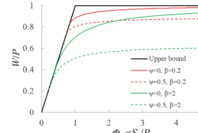
Equations (15) and (17) provide W_P as a function of8scwith

two parameters (ψandβ). Figure 2 plots Eqs. (15) and (17) forψ=0 and 0.5 whenβ=0.2 and 2. As we can see,W_P de-creases asβincreases for given values ofψand8sc, and W_P

decreases asψincreases for given values ofβ and8sc,

im-plicating that the soil wetting ratio decreases with the degree of initial saturation under a given the soil storage index.

4 Comparison between the SCS-CN model and the VIC type of model

The SCS-CN model with the parameterization of the ratio be-tween initial wetting and total wetting is compared with the VIC type of saturation excess runoff model. In Sects. 2 and 3, we derived W_P as a function of8sc based on the SCS-CN

method and the VIC type of model, which uses a generalized

Figure 2. The impact of β and the degree of initial storage

(ψ=S0/Sb)on the soil wetting ratio(W/P ).

Pareto distribution to describe the spatial distribution of stor-age capacity. The SCS-CN method is a function of storstor-age capacitySp, but the VIC type of model is a function of

stor-age capacitySpand the degree of initial saturation S_S0

b. As a

result, the function of W_P ∼Sp

P for the SCS-CN method has

only one parameter (ε), but it has two parameters (β andψ) for the VIC type of model.

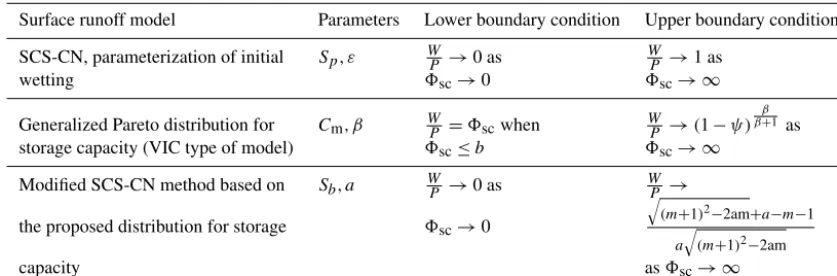
Table 1 shows the boundary conditions for the relation-ships between W_P and 8sc from the SCS-CN method and

the VIC type of model. The lower boundary of the SCS-CN method with parameterεis W_P →0 as 8sc→0. However,

for the VIC type of model, W_P =8sc when8sc≤b. For the

SCS-CN method,Wreaches its maximum (Sp) when rainfall

reaches infinity, while for the VIC type of model,Wreaches its maximum value (Sp) when rainfall reaches a finite

num-ber(Cm−C0). In other words, for the SCS-CN method, the

entire catchment becomes saturated when rainfall reaches in-finity, while for the VIC-type model, the entire catchment becomes saturated when rainfall reaches a finite number.

As shown in Table 1, the upper boundary of the SCS-CN method (with parameterε) is 1. However, for the VIC type of model, the upper boundary is(1−ψ )

β

β+1 _{instead of 1. This is}

due to the effect of initial storage in the VIC type of model. When initial storage is 0 (i.e.,ψ=0), the wetting ratio W_P for the VIC type of model has the same upper boundary con-dition as the SCS-CN method.

5 Unification of the SCS-CN method and the VIC type of model

Based on the comparison between the SCS-CN method and the VIC type of model, a new distribution function is pro-posed in this section for describing the spatial distribution of soil water storage capacity, which unifies the SCS-CN method and the VIC type of model. As discussed in Sect. 4, the upper boundary condition of the SCS-CN model (i.e.,

W

stor-Table 1.The boundary conditions of the functions for relating the wetting ratio

W P

to the soil storage index(8sc): (1) the SCS-CN method, (2) the VIC type of model, and (3) the modified SCS-CN method based on the proposed new distribution for the VIC type of model.

Surface runoff model Parameters Lower boundary condition Upper boundary condition

SCS-CN, parameterization of initial Sp, ε W_P →0 as W_P →1 as

wetting 8sc→0 8sc→ ∞

Generalized Pareto distribution for Cm, β W_P =8scwhen W_P →(1−ψ )

β β+1 _as

storage capacity (VIC type of model) 8sc≤b 8sc→ ∞

Modified SCS-CN method based on Sb, a W_P →0 as W_P →

the proposed distribution for storage 8sc→0

q

(m+1)2−2am+a−m−1

a q

(m+1)2−2am

capacity as8sc→ ∞

age. This upper boundary condition needs to be modified by including the effect of initial storage so that the limit of W_P as8sc→ ∞is dependent on the degree of initial saturation

like the VIC type of model. However, the lower boundary condition of the VIC model needs to be modified so that the lower boundary condition follows that ofW_P →0 as8sc→0

like the SCS-CN method. Through these modifications, the SCS-CN method and the VIC type of saturation excess runoff model can be unified from the functional perspective of the soil wetting ratio.

Based on the comparison one may have the following questions. (1) Can the SCS-CN method be derived from the VIC type of model by setting initial storage to 0? (2) If yes, what is the distribution function for soil water storage capac-ity? Once we answer these questions, a modified SCS-CN method considering initial storage explicitly can be derived as a saturation excess runoff model based on a distribution function of water storage capacity, and it unifies the SCS-CN method and the VIC type of model. In this section, a new distribution function is proposed for describing the spa-tial variability of soil water storage capacity, from which the SCS-CN method is derived as a VIC type of model.

5.1 A new distribution function

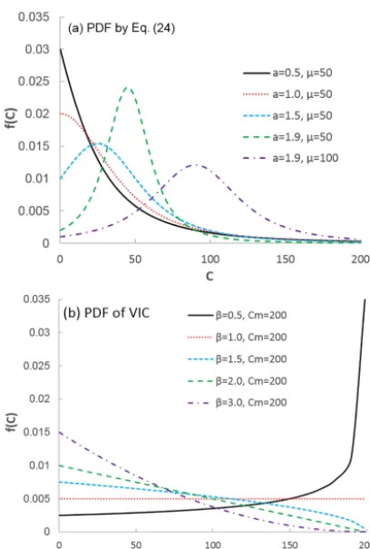
The probability density function (PDF) of the new distribu-tion for describing the spatial distribudistribu-tion of water storage capacity is represented by

f (C)= (2−a) µ

2

(C+µ)2−2aµC3/2

, (19)

whereC is the point-scale water storage capacity and sup-ported on a positive semi-infinite interval (C≥0),a is the shape parameter and its range is 0< a <2, andµis the mean of the distribution (i.e., the scale parameter). Figure 3a plots the PDFs for five sets of shape and scale parameters. When a≤1, the PDF monotonically decreases with the increase of C; i.e., the peak of the PDF occurs atC=0, while when

a >1 the peak of the PDF occurs atC >0 and the location of the peak depends on the values ofaandµ. For compar-ison, Fig. 3b plots the PDF for the VIC model. As shown by the solid black curve in Fig. 3b, when 0< β <1, f (C) approaches infinity asC→Cm. It is a uniform distribution

when β=1. The peak of the PDF occurs at C=0 when β >1. Therefore, the peak of the PDF for the VIC model occurs atC=0 orCm.

The cumulative distribution function (CDF) corresponding to the proposed PDF is obtained by integrating Eq. (19):

F (C)=1−1 a +

C+(1−a) µ a

q

(C+µ)2−2aµC

. (20)

Figure 4a plots the CDFs corresponding to the PDFs in Fig. 3a. For comparison, Fig. 4b plots the CDFs correspond-ing to the PDFs in Fig. 3b. The storage capacity distribu-tion curve for the proposed distribudistribu-tion is concave up for a≤1 and S shaped for a >1 (Fig. 4a), while the storage capacity distribution curve for the VIC model is concave up forβ >1 and concave down for 0< β <1 (Fig. 4b). The S shape of the CDF (Fig. 4a) is more significant with a higher value ofa (e.g.,a=1.9). For a smaller value ofa, the dif-ference between the new PDF and the VIC type of model be-comes smaller. The proposed distribution can fit the S shape of the cumulative distribution for storage capacity which is observed from soil data (Huang et al., 2003), but the general-ized Pareto distribution of the VIC type of model is not able to fit the S shape of the CDF.

5.2 Deriving the SCS-CN method from the proposed distribution function

distri-Figure 3.The probability density functions (PDFs) with different parameter values: (a)the proposed PDF represented by Eq. (24) and(b)the generalized Pareto distribution of the VIC model, i.e., Eq. (25).

bution:

µ=Sb. (21)

For a given C, the catchment-scale storage S can be computed by S=RC

0 [1−F (x)] dx (Moore, 1985). From

Eq. (20), we obtain

S=C+Sb−

p

(C+Sb)2−2aSbC

a . (22)

For a rainfall–runoff event, the average initial storage at the catchment scale is denoted asS0and the corresponding value

ofC is denoted asC0. SubstitutingS0andC0into Eq. (22),

we obtain m=ψ (2−aψ )

2(1−ψ ) , (23)

whereψ=S0

Sb is defined in Eq. (12) andm

=C0

Sb.

The rainfall in the catchment is assumed to be spatially uniform and the rainfall depth is denoted asP. If the spatial distribution of rainfall is not uniform, the method is applied to sub-catchments where the effect of spatial variability of rainfall is negligible. The average storage at the catchment

Figure 4.The cumulative distribution functions (CDFs) with differ-ent parameter values:(a)the proposed distribution function repre-sented by Eq. (26) and(b)the generalized Pareto distribution of the VIC model represented by Eq. (13).

scale after infiltration is computed by substitutingC=C0+

P into Eq. (22):

S1=

C0+P+Sb− p

(C0+P+Sb)2−2aSb(C0+P )

a . (24)

The soil wetting is computed as the difference betweenS1

andS0:

W=

P+p(C0+Sb)2−2aSbC0− p

(C0+P+Sb)2−2aSb(C0+P )

a . (25)

DividingP on both sides of Eq. (25) and substitutingm=

C0

Sb, we obtain

W P =

1+Sb

P

p

(m+1)2−2am− r

1+(m+1)Sb

P

2 −2amSb

P

2 −2aSb

P

a . (26)

Substituting Eq. (13) into Eq. (26), we obtain W

1+ √

(m+1)2−2am 1−ψ 8sc−

r

1+m+1 1−ψ8sc

2

−2am8sc 1−ψ

2

− 2a

1−ψ8sc

a . (27)

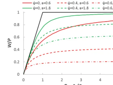
Figure 5 plots Eq. (27) forψ=0, 0.4, and 0.6 whena=0.6 and 1.8. As we can see, W_P increases witha for given val-ues ofψand8sc, and W_P decreases withψfor given values

of a and8sc, which is consistent with the VIC model and

implicates that the soil wetting ratio decreases with the de-gree of initial saturation under a storage index. As shown in Fig. 5, Eq. (27) satisfies the lower boundary of the SCS-CN method and the upper boundary of the VIC model. Specif-ically, Eq. (27) satisfies the following boundary conditions (see Appendix D for details) shown in Table 1:

lim

8sc→0

W

P =0, (28a)

lim

8sc→∞

W P =

p

(m+1)2−2am+a−m−1 ap(m+1)2−2am

. (28b)

When the effect of initial storage is negligible (i.e.,ψ=0),

Sb

P =8sc from Eq. (13) and m=0 from Eq. (23). Then,

Eq. (27) becomes

W P =

1+Sb

P −

r

1+Sb

P

2

−2aSb

P

a . (29)

Equation (29) is same as Eq. (8) witha=2ε (2−ε). We can obtain the following equation from Eq. (29) (see Appendix E for a detailed derivation):

Q P−εW =

W−εW Sb−εW

, (30)

whereεW is defined as initial abstraction (Wi)in the

SCS-CN method. SinceSb=Spwhenψ=0, Eq. (30) is same as

Eq. (2), i.e., the proportionality relationship of the SCS-CN method.

Equation (27) is derived from the VIC-type model by us-ing Eq. (20) to describe the spatial distribution of soil water storage capacity. From this perspective, Eq. (27) is a satura-tion excess runoff model. Since Eq. (27) becomes the SCS-CN method when initial storage is negligible, Eq. (27) is the modified SCS-CN method which considers the effect of initial storage on runoff generation explicitly. Therefore, the new distribution function represented by Eq. (20) unifies the SCS-CN method and the VIC type of model.

Bartlett et al. (2016a) developed an event-based proba-bilistic storage framework including a spatial description of prethreshold and threshold-excess runoff, and the framework has been utilized for unifying TOPMODEL, VIC, and SCS-CN (Bartlett et al., 2016b). The extended SCS-SCS-CN method (SCS-CNx) from the probabilistic storage framework is de-rived given the following assumptions: (1) the spatial distri-bution of rainfall is exponential, (2) the spatial distridistri-bution of the soil moisture deficit is uniform, and (3) the spatial distri-bution of storage capacity is exponential. When prethreshold

Figure 5.The effects of the degree of initial storage (ψ=0, 0.4, and 0.6) and shape parameter (a=0.6 and 1.8) on soil wetting in the modified SCS-CN method derived from the proposed distribution function for soil water storage capacity.

runoff is 0 (i.e., there is only threshold-excess or saturation excess runoff), the SCS-CNx method leads to the SCS-CN method without the initial abstraction term (i.e., there is no εW term in Eq. 30). In this paper, the new probability dis-tribution function is used for storage capacity in the VIC model in which the spatial distribution of precipitation is as-sumed to be uniform. The obtained equation for saturation excess runoff leads to the exact SCS-CN method as shown in Eq. (30).

This research started with the following research ques-tion: if the SCS-CN method is a saturation excess runoff generation model, what is the distribution function of soil water storage capacity? Wang and Tang (2014) showed that Eq. (29) is derived from the proportionality relationship of the SCS-CN method, i.e., Eq. (30). From the comparison of boundary conditions between the SCS-CN method and the VIC type of model discussed in Sect. 4, it is observed that Eq. (29) does not include initial soil water storage, and the derived one from the distribution function will include initial soil water storage (e.g., Eq. 26). However, Eq. (29) can be viewed as the result ofS0=0, and W for Eq. (29) can be

written as

W=

P

Z

0

[1−F (x)] dx. (31)

From Eq. (29), one obtains W=P +Sb−

p

(Sb+P )2−2aP Sb

a . (32)

Substituting Eq. (32) into Eq. (31), one obtains P +Sb−

p

(Sb+P )2−2aP Sb

a =

P

Z

0

[1−F (C)] dC. (33)

Figure 6. (a)The effects of average storage capacity and initial stor-age on the rainfall–runoff relation and(b)the effects of average stor-age capacity and shape parameter on the rainfall–runoff relation.

5.3 Surface runoff of the unified SCS-CN and VIC model

From the unified SCS-CN and VIC model (i.e., Eq. 26), sur-face runoff (Q) can be computed as

Q= (a−1) P−Sb

p

(m+1)2_−2am+q_[P+(m+1)S

b]2−2amSb2−2aSbP

a . (34)

The parameter mis computed by Eq. (23) as a function of ψ anda. Equation (34) represents surface runoff as a func-tion of precipitafunc-tion (P), average soil water storage capacity (Sb), the shape parameter of the storage capacity

distribu-tion (a), and initial soil moisture (ψ). Fig. 6 plots Eq. (34) under different values ofP,Sb,a, andψ. Figure 6a shows

the effects of Sb and ψ on the rainfall–runoff relationship

with a given shape parameter of a=1.9. The solid lines show the rainfall–runoff relations with zero initial storage (ψ=0) and the dashed lines show the rainfall–runoff rela-tions withψ=0.2. Given the same amount of precipitation and storage capacity, wetter soil (ψ=0.2) generates more surface runoff than drier soil (ψ=0), and the difference of runoff is higher for watersheds with larger average storage capacity. Figure 6b shows the effects of Sb and a on the

rainfall–runoff relationship with a given initial soil moisture (ψ=0.2). The solid lines show the rainfall–runoff relations fora=1.9 and the dashed lines show the rainfall–runoff re-lations fora=1.2. As we can see, the shape parameter af-fects the runoff generation significantly for watersheds with larger average storage capacity.

In the SCS-CN method, surface runoff is computed as Q=(P−0.2Sb)2

P+0.8Sb . The effect of initial soil moisture on runoff

is considered implicitly by varying the curve number for nor-mal, dry, and wet conditions depending on the antecedent moisture condition. In the unified SCS-CN model shown in Eq. (34), the effect of initial soil moisture is explicitly in-cluded throughψ, which is the ratio between average initial water storage and average storage capacity. In the SCS-CN method, the value of initial abstractionWi is parameterized

as a function of average storage capacity; i.e.,Wi=0.2Sb. In

the unified SCS-CN model shown in Eq. (34),Wi is

depen-dent on the shape parametera. Therefore, the unified SCS-CN model extends the original SCS-SCS-CN method for includ-ing the effect of initial soil moisture explicitly and estimatinclud-ing the parameter for initial abstraction.

6 Conclusions

In this paper, the SCS-CN method and the saturation ex-cess runoff models based on distribution functions (e.g., VIC model) are presented in terms of soil wetting (i.e., infiltra-tion). Like the Budyko framework, the relationship between the soil wetting ratio and the soil storage index is obtained for the SCS-CN method and the VIC type of model. It is found that the boundary conditions for the obtained functions do not fully match. For the SCS-CN method, the soil wetting ra-tio approaches 1 when the soil storage index approaches in-finity, and this is due to the limitation of the SCS-CN method; i.e., the initial soil moisture condition is not explicitly repre-sented in the proportionality relationship. However, for the VIC type of model, the soil wetting ratio equals the soil stor-age index when the soil storstor-age index is lower than a certain value, and this is due to the finite bound of the distribution function of storage capacity.

following boundary conditions: when the storage index ap-proaches 0, the soil wetting ratio apap-proaches 0; when the storage index approaches infinity, the soil wetting ratio ap-proaches a certain value (≤1) depending on the initial stor-age (e.g., at the beginning of a rainfall event, runoff is gen-erated at the initially saturated areas, Yu et al., 2001; Gao et al., 2018). Meanwhile, the model becomes the exact SCS-CN method when initial storage is negligible. Therefore, the new distribution function for soil water storage capacity explains the SCS-CN method as a saturation excess runoff model and unifies the SCS-CN method and the VIC type of model for surface runoff modeling.

Future potential work could test the performance of the proposed new distribution function for quantifying the tial distribution of storage capacity by analyzing the spa-tially distributed soil data. On the one hand, the distribu-tion funcdistribu-tions of the probability distributed model (Moore, 1985), VIC model, and Xinanjiang model could be replaced by the new distribution function and the model performance would be further evaluated. On the other hand, the extended SCS-CN method (i.e., Eq. 27), which includes initial stor-age explicitly, could be used for surface runoff modeling in the SWAT (Soil and Water Assessment Tool) model, and the model performance would be evaluated.

Data availability. This paper is a theoretical analysis and does not

Appendix A

The potential for continuing wetting is called potential max-imum retention and is denoted bySm=Sp−Wi.Smis

com-puted as a function of curve number which is dependent on land use–land cover and soil permeability. The ratio between Wi andSmin the SCS curve number method is denoted by

λ= Wi

Sp−Wi, and then the ratio between initial soil wetting and

storage capacity is computed by

Wi

Sp

= λ

1+λ. (A1)

The value of λvaries in the range of 0≤λ≤0.3, and a value of 0.2 is usually used (Ponce and Hawkins, 1996). Sub-stituting Eq. (A1) into Eq. (6) leads to

W P =

1− λ

1+λ

2

8sc

1− 2λ

1+λ+8 −1 sc

. (A2)

Equation (A2) is plotted in Fig. 1 for λ=0.1 and 0.3. As we can see, the range of 8sc is dependent on the

pa-rameterλ. SinceWi≤P,8sc is in the range of

h

0,1+1

λ

i

. Equation (A2) satisfies the following boundary conditions:

W

P →0 as8sc→0 and W

P →1 as8sc→ λ+1

λ . Whenλ→

0, Eq. (A2) becomes W

P = 1 1+8−sc1

. (A3)

Equation (A3) is the lower bound forW_P based on this param-eterization scheme.

Appendix B

SubstitutingW=S1−S0into Eq. (16), wetting is computed

by

W =Sb

"

1−

1−P+C0 Cm

β+1#

−S0. (B1)

The following equation is obtained by dividing P on both sides of Eq. (B1):

W P =

Sb−S0

P − Sb

P

1−P+C0 Cm

β+1

. (B2)

Substituting C0

Cm =1−

1−S0

Sb

_β+1₁

into Eq. (B2), we obtain

W P =

Sb−S0

P −

Sb

P 1− P Cm − " 1− 1−S0

Sb _β+11#!

β+1

. (B3)

Substituting Eq. (10) into Eq. (B3), we obtain

W P =

Sb−S0

P −     _S

b−S0

P

_β+11

−

Sb

P

−_ββ₊₁

β+1



  

β+1

. (B4)

Substituting Eqs. (5) and (13) into Eq. (B4), we obtain

W

P =8sc−

    8 1

β+1

sc −

8sc

1−ψ

−_β+β1

β+1



  

β+1

, (B5)

which leads to W

P =8sc

1−

1−b8−_sc1

β+1

, (B6)

wherebis defined in Eq. (14).

Appendix C

lim

8sc→∞

W

P =8sclim→∞

8sc

1−1−b8−_sc1β +1

(C1) The right-hand side of Eq. (C1) is rewritten as

lim

8sc→∞

8sc

1−1−b8−_sc1

β+1

=

lim

8sc→∞

1− 1−b8−_sc1β+1

8−sc1

. (C2)

Since lim8sc→∞1− 1−b8

−1 sc

β+1

=0 and

lim8sc→∞8

−1

sc =0, we apply the L’Hospital’s rule,

lim

8sc→∞ h

1− 1−b8−_sc1β+1i0

8−sc1

0

=

lim

8sc→∞

b(β+1)1−b8−_sc1

β

. (C3)

Since lim8sc→∞ 1−b8

−1 sc

β

=1, the limit for W_P is ob-tained as follows:

lim

8sc→∞

W

P =b (β+1) . (C4) Substituting Eq. (14) into Eq. (C4), we obtain

lim

8sc→∞

W

P =(1−ψ )

β

Appendix D

lim

8sc→∞

W

P =8sclim→∞ 1+

√

(m+1)2−2am 1−ψ 8sc−

r

1+m₁₋+_ψ18sc

2

−2am8sc 1−ψ

2 −₁2₋a_ψ8sc

a (D1)

Multiplying

1+

p

(m+1)2−2am 1−ψ 8sc

+

s

1+m+1

1−ψ8sc

2

−2am

₈ sc

1−ψ

2

− 2a

1−ψ8sc (D2)

with the denominator and numerator of the right-hand side Eq. (D1) leads to

lim

8sc→∞

W

P = 1 a8sclim→∞ 2

q

(m+1)2−2am

1−ψ 8sc−2(m1−+ψ1)8sc+12−aψ8sc 1+

q

(m+1)2−2am 1−ψ 8sc+

r

1+m+1

1−ψ8sc

2

−2am8sc 1−ψ

2 − 2a

1−ψ8sc

.

(D3) Dividing8scin the denominator and numerator, we obtain

lim

8sc→∞

W P =

1

a (1−ψ )8sclim→∞ 2

q

(m+1)2−2am−2(m+1)+2a

1

8sc+ q

(m+1)2−2am 1−ψ +

r

1

8sc+

m+1 1−ψ

2

−2am₁₋1_ψ2− 2a

(1−ψ )8sc

.

(D4) Therefore, the limit of W_P as8sc→ ∞is

lim

8sc→∞

W P =

p

(m+1)2−2am+a−m−1 ap(m+1)2−2am

. (D5)

Appendix E

Substitutinga=2ε (2−ε)into Eq. (29), one can obtain

W P =

1+Sb

P −

r

1+Sb

P

2

−4ε (2−ε)Sb

P

2ε (2−ε) . (E1)

Equation (E1) is the solution of the following quadratic func-tion:

ε (2−ε)

_W

P

2

−

1+Sb P

_W

P + Sb

P =0. (E2) MultiplyingP2on both sides of Eq. (E2), Eq. (E2) becomes ε (2−ε) W2−(P+Sb) W+SbP =0. (E3)

Equation (E3) can be written as the following one: P−W

P −εW =

W−εW Sb−εW

. (E4)

SubstitutingQ=P−Winto Eq. (E4), we obtain the propor-tionality relationship of the SCS-CN method:

Q P −εW =

W−εW Sb−εW

Competing interests. The authors declare that they have no conflict of interest.

Acknowledgements. This research was funded in part under award

CBET-1804770 from the National Science Foundation (NSF) and the United States Geological Survey (USGS) Powell Center Working Group Project “A global synthesis of land-surface fluxes under natural and human-altered watersheds using the Budyko framework”. The authors would also like to thank the Associate Editor and three reviewers for their constructive comments and suggestions that have led to substantial improvements over an earlier version of the manuscript.

Edited by: Zhongbo Yu

Reviewed by: three anonymous referees

References

Bartlett, M. S., Parolari, A. J., McDonnell, J. J., and Porporato, A.: Beyond the SCS-CN method: A theoretical framework for spa-tially lumped rainfall-runoff response, Water Resour. Res., 52, 4608–4627, https://doi.org/10.1002/2015WR018439, 2016a. Bartlett, M. S., Parolari, A. J., McDonnell, J. J., and

Por-porato, A.: Framework for event-based semidistributed modeling that unifies the SCS-CN method, VIC, PDM, and TOPMODEL, Water Resour. Res., 52, 7036–7052, https://doi.org/10.1002/2016WR019084, 2016b.

Beven, K.: Rainfall-Runoff Modelling: The Primer, 2nd Edn., Wiley-Blackwell, Chichester, UK, 2012.

Beven, K. and Kirkby, M. J.: A physically based, variable contribut-ing area model of basin hydrology, Hydrol. Sci. J., 24, 43–69, 1979.

Bras, R. L.: Hydrology: an introduction to hydrologic science, Ad-dison Wesley Publishing Company, Reading, MA, 1990. Budyko, M. I.: Climate and Life, 508 pp., Academic Press, New

York, 1974.

Chen, X., Alimohammadi, N., and Wang, D.: Modeling interannual variability of seasonal evaporation and storage change based on the extended Budyko framework, Water Resour. Res., 49, 6067– 6078, https://doi.org/10.1002/wrcr.20493, 2013.

Easton, Z. M., Fuka, D. R., Walter, M. T., Cowan, D. M., Schnei-derman, E. M., and Steenhuis, T. S.: Re-conceptualizing the soil and water assessment tool (SWAT) model to predict runoff from variable source areas, J. Hydrol., 348, 279–291, 2008.

Gao, H., Birkel, C., Hrachowitz, M., Tetzlaff, D., Soulsby, C., and Savenije, H. H. G.: A simple topography-driven and calibration-free runoff generation module, Hydrol. Earth Syst. Sci. Discuss., https://doi.org/10.5194/hess-2018-141, in review, 2018. Hooshyar, M. and Wang, D.: An analytical solution of Richards’

equation providing the physical basis of SCS curve number method and its proportionality relationship, Water Resour. Res., 52, 6611–6620, https://doi.org/10.1002/2016WR018885, 2016. Huang, M., Liang, X., and Liang, Y.: A transferability study

of model parameters for the variable infiltration capac-ity land surface scheme, J. Geophys. Res., 108, 8864, https://doi.org/10.1029/2003JD003676, 2003.

Liang, X., Lettenmaier, D. P., Wood, E. F., and Burges, S. J.: A sim-ple hydrologically based model of land surface water and energy fluxes for general circulation models, J. Geophys. Res.-Atmos., 99, 14415–14428, 1994.

Lyon, S. W., Walter, M. T., Gérard-Marchant, P., and Steenhuis, T. S.: Using a topographic index to distribute variable source area runoff predicted with the SCS curve – number equation, Hydrol. Process., 18, 2757–2771, 2004.

Mishra, S. K. and Singh, V. P.: Another look at SCS-CN method, J. Hydrol. Eng., 4, 257–264, 1999.

Mockus, V.: National Engineering Handbook Section 4, Hy-drology, NTIS, available at: https://directives.sc.egov.usda. gov/OpenNonWebContent.aspx?content=18393.wba (last ac-cess: 19 December 2018), 1972.

Moore, R. J.: The probability-distributed principle and runoff pro-duction at point and basin scales, Hydrol. Sci. J., 30, 273–297, 1985.

Ponce, V.: Notes of my conversation with Vic Mockus, unpub-lished material, available at: http://mockus.sdsu.edu/ (last ac-cess: 29 September 2017) 1996.

Ponce, V. M. and Hawkins, R. H.: Runoff curve number: has it reached maturity?, J. Hydrol. Eng., 1, 9–20, 1996.

Porporato, A., Daly, E., and Rodriguez-Iturbe, I.: Soil Water Bal-ance and Ecosystem Response to Climate Change, Am. Nat., 164, 625–632, 2004.

Sivapalan, M., Beven, K., and Wood, E. F.: On hydrologic similar-ity: 2. A scaled model of storm runoff production, Water Resour. Res., 23, 2266–2278, 1987.

Steenhuis, T. S., Winchell, M., Rossing, J., Zollweg, J. A., and Walter, M. F.: SCS runoff equation revisited for variable-source runoff areas, J. Irrig. Drain. Eng., 121, 234–238, 1995.

Tang, Y. and Wang, D.: Evaluating the role of watershed properties in long-term water balance through a Budyko equation based on two-stage partitioning of precipitation, Water Resour. Res., 53, 4142–4157, https://doi.org/10.1002/2016WR019920, 2017. Wang, D. and Tang, Y.: A one-parameter Budyko model

for water balance captures emergent behavior in Darwinian hydrologic models, Geophys. Res. Lett., 41, 4569–4577, https://doi.org/10.1002/2014GL060509, 2014.

Wang, D., Zhao, J., Tang, Y., and Sivapalan, M.: A thermo-dynamic interpretation of Budyko and L’vovich formulations of annual water balance: Proportionality hypothesis and maxi-mum entropy production, Water Resour. Res., 51, 3007–3016, https://doi.org/10.1002/2014WR016857, 2015.

Wood, E. F., Lettenmaier, D. P., and Zartarian, V. G.: A land – surface hydrology parameterization with subgrid variability for general circulation models, J. Geophys. Res.-Atmos., 97, 2717– 2728, 1992.

Yu, B.: Theoretical justification of SCS method for runoff estima-tion, J. Irrig. Drain. Eng., 124, 306–310, 1998.

Yu, Z., Carlson, T. N., Barron, E. J., and Schwartz, F. W.: On evaluating the spatial-temporal variation of soil moisture in the Susquehanna River Basin, Water Resour. Res., 34, 1313–1326, 2001.

Zhao, R.: Flood forecasting method for humid regions of China, East China College of Hydraulic Engineering, Nanjing, China, 1977.