An Effective Cost Measurement Model for Cloud Storage Computing

© 2016, IRJET | Impact Factor value: 4.45 | ISO 9001:2008 Certified Journal | Page 406

An Effective Cost Measurement Model for Cloud Storage Computing

Md. Mahmudul Hasan

_{, Md. Sorowar Hossain}

1, 2

_{Department of Computer Science and Engineering, Pabna University of Science and Technology,}

Pabna, Bangladesh

---***---Abstract –

contents is rising with the increasing availability of internet across the world. Cloud storage computing offers instant, dominant, cost-effective, and high performance storage service to the growing community. The cost associated to fulfill the demand varies based on the choice of the customer. In this paper, we identify such cost factors to build a two-step cost estimation model for cloud storage computing. We aim to investigate cost factors to build a mathematical model and obtain an idea how much they affect on the expense for cloud storage computing. In the first step, we investigate the contributing effect of each factor towards the total cost and build a linear relationship using Reduced Row Echelon Form. In the second step, we are motivated to improve the model further using an evolutionary algorithm. From the evidence of the final result we observe that the proposed model performs significantly well.

Key Words: Cost Estimation, Cloud Storage, Cost Factors,

Amazon S3, Genetic Algorithm.

1. INTRODUCTION

The increasing popularity of cloud computing has risen more interests among IT organizations to utilize appealing computing services with the growing facility and easy getting of internet connection. The rapid, ever sophisticated technological development of cloud services has made the computing resources less costly but even more powerful and universal.

Cloud storage, a major revolutionary service, is also increasingly important as users are more tends to store their regular files, data and contents to remote servers that they can access, change and share them from anywhere of the world. The pay-as-you-go formula in cloud computing has reduced the cost of computing services significantly as users need no purchase of complete physical machine instantly [1]. They can consume leveraged storage services from potential storage service providers such as Amazon S3, Microsoft Azure, Google Drive, Dropbox, Tresorit, pCloud, OneDrive and so on.

As cloud is defined by multiple remote servers located around the globe, the storage of user contents and data is distributed to different servers placed decentralized. Service providers establish giant data centers consisting of many Virtual Machines (VMs) and increase the reliability via

storage redundancy and elasticity. The cost associated with this growing advantage is also piling up. In addition, storing data involves requests for inbound and outbound data that also cost much when users migrate their data to other providers [2].

In literature, several cost-benefit analyses have been conducted over years where the main focus has been the performance measurement of applications in cloud storage in terms of accessing data [3], operating parallel programs [4], providing security [5] and analyzing scientific data in popular cloud storage services such as Amazon EC2 and S3 [6]. In [7], the authors identified that some of the computational factors such as data transfer in and out are more important than the storage size itself for measuring the cost. Amazon S3 is a popular storage service that has been a basic model in many studies related to the cost analysis. In this study, we refer to factors found in Amazon S3 Monthly Calculator (AMC) [11] related to cloud storage computing costs and collected a set of relevant data. We then build a stepwise model associating these cost factors. At first, we investigate a linear relationship among cost factors that drive the total cost calculated from the AMC. Later, we attempt to apply an evolutionary algorithm to calibrate the findings for further improvement. We also compare the performances in each step and validate the proposed model with some test cases.

In the remainder of this paper, we first define the cloud storage computing and describe associated cost factors in section 2. In section 3, we describe our research methodology towards building the cost measurement model. Section 4 and section 5 explains the relevant background theory and the implementation of the model respectively. The model is evaluated and validated in section 6 followed by the concluding statements in section 7.

2. CLOUD STORAGE COMPUTING

2.1 Definition

© 2016, IRJET | Impact Factor value: 4.45 | ISO 9001:2008 Certified Journal | Page 407

on-demand high quality services that can be managed via configurable computing resources [10]. Computing means the manipulation of requests for storing and pulling data in cloud servers.

1.2 Identifying Cost Factors

From the literatures, we observe that several cost factors are involved in the cost diversity happened in individual studies. Many of the factors are found in the Amazon S3 Monthly Calculator [11].

a. Standard Storage (SS): It refers to the storage for frequently accessed data that offers high durability (99.999999%), availability (99.99%) and performance with maintaining the SLA (Service Level Agreements) [12]. b. Standard - Infrequent Access Storage (Standard IA): For accessing less frequent data Amazon S3 offers fewer prices with same performance as standard but provides rapid access when necessary. This class is feasible to consume for long term storage, backups and data storage for disaster recovery [12].

c. Reduced Redundancy Storage (RRS): This class of storage offers cost-effective price for distributing or sharing content. The types of data that can be reproduced very easily are suitable for this storage class [13].

d. Data Transfer: Transferring data involves requests for storing (inbound) data in cloud servers and pulling (outbound) data from the server that are important in cost measurement process [2]. Amazon S3 offers no cost for inbound data but has pricing classes for outbound data [14].

In this study, we use 5 factors for building the cost model: Standard Storage (SS), Standard IA Storage (SIAS), Reduced Redundancy Storage (RRS), Data Transfer Out (DTO) and a subclass of data transfer, Inter-Region Data Transfer Out (IRDTO) that also has effect on total pricing [11].

3. RESEARCH METHODOLOGY

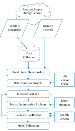
We aim to build a two-step cost measurement model using the contributing factors identified in previous section. Fig -1 depicts the proposed architecture. Prior to build the model we prepare a data set containing values of each factor and the corresponding measured cost using the monthly calculator.

3.1 Data Collection

In the data collection process, we input random but uniform range of data into the form controls. The units of storage amount are of three kinds: GB (Giga Bytes), TB (Tera Bytes) and PT (Peta Bytes). In this study, we consider data ranges in GB only. It can be noted that if we choose data values of tiny range (1-5 GB) then the total cost becomes very tiny that are not suitable for our analysis. This is

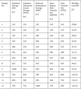
acceptable because the S3 service provides very tiny cost value for each class of storage per GB. It is possible for users to demand tiny amount but for analytical purposes we consider large amounts, greater than 100GB, in the data collection process. It is also noted that a tab located at the top of the page that says ‘Estimate of your Monthly Bill ($xx.xx)’ presents the total cost calculated from the given input. We collect 12 such samples as our analytical data consisting of values ranges from 100 GB to 1000 GB. Table 1 represents the collected data from the AMC. It is noted that, we do not consider the free tier discount as the offer expires after 12 months.

Fig -1: Proposed Architecture Amazon Simple Storage Service

Data Collection Monthly

Calculator

Identify Factors

Build Linear Relationship

Determine Coefficients

Row Echelon

Form

Measure Cost and Performance

Devise Optimization Problem

Error Minimize

Calibrate Coefficient Search Criteria

© 2016, IRJET | Impact Factor value: 4.45 | ISO 9001:2008 Certified Journal | Page 408

3.2 First Step Model

At first step, we aim to establish a linear relationship between factors, and the total cost. The identified five factors (xi , i = 1 to n, n= 5) are considered as independent variables of the linear equation. The calculated cost (C) is counted as the dependent variable. Equation (1) represents the linear equation of our proposed model.

C = (1)

where ai refers to the coefficient of i-th factor, xi.

Table -1: Samples Collected from Amazon S3 Monthly Calculator

Sample

No. Standard Storage (SS)

[x1]

Standard Infrequent Access Storage (SIAS) [x2]

Reduced Redundancy Storage (RRS)

[x3]

Inter-Region Data Transfer Out (IRDTO)

[x4]

Data Transfer Out (DTO)

[x5]

Monthly Cost Bill

[C]

1 115 135 125 145 165 25.80

2 165 145 130 120 115 22.55

3 155 135 180 220 145 28.02

4 345 235 350 120 255 46.95

5 285 335 210 385 315 53.74

6 555 445 250 500 400 74.13

7 650 700 565 355 500 93.82

8 625 755 765 595 425 96.61

9 1000 465 550 850 350 97.43

10 750 820 700 665 800 134.76

11 850 585 250 500 750 116.23

12 750 735 1000 750 550 120.10

When solving this linear equation, a coefficient value for each factor determines how much that factor drives the total cost alongside other factors in effect. We use a well known process, Reduced Row Echelon Form (RREF) used in linear algebra, to solve the proposed linear equation. At the end of this step, we expect to obtain a set of values of five coefficients that insights us how they are contributing to the final cost. We recalculate the total cost from the linear equation using the coefficient and collected data. Later, we compare this measured cost with the original cost collected from the AMC and measure the performance.

3.3 Second Step Model

In this step, we aim to improve the performance of the proposed first step model if the linear system turns out to be a weak solution. We apply an evolutionary algorithm, GA (Genetic Algorithm) to calibrate the coefficients obtained from the first step model. The idea behind taking the coefficients from previous step is to GA to search feasible solutions within smaller boundary. At the end of this step, we expect to obtain a set of five calibrated coefficients and a modified total cost measured by GA. Finally, we compare models obtained from each step and measure the performance of the models to present the final acceptable model. The evaluation of each model is conducted by some model evaluation criteria presented in the next subsection.

3.4 Model Evaluation Criteria

We validate each step of models by four evaluation criteria: Mean Absolute Error (MAE), Magnitude of Relative Error (MRE), Mean MRE (MMRE) and Mean Absolute Percentage Error (MAPE).

a. MAE: Mean Absolute Error (MAE) is very popular in evaluating data analytical models. It represents how a new predictive model is deviated from the original system based on a number of sample data analyzed to build the new model. The MAE can be expressed as

where n is the number of observations on which the errors are measured. In errors |ei| = |fi - yi|, fi is the measured value and yi is the original value from the dataset.

b. MRE and MMRE: The Magnitude of Relative Error (MRE) and Mean Magnitude of Relative Error (MMRE) are another popular validation process used in statistical and optimization studies. MRE tells us how the new predictive model is deviated from the original system with respect to the magnitude of each sample in given set of data. The common form of MRE

where Z is the measured value and Y is the actual value from the dataset. MMRE is the mean value of MRE and it takes into account the numerical value of every observation in the data distribution, and is sensitive to individual predictions with large MREs.

© 2016, IRJET | Impact Factor value: 4.45 | ISO 9001:2008 Certified Journal | Page 409

MAPE

where Ai is the actual value and Fi is the forecast value. It is expressed as percentage (%) error. It provides the idea of a bias of predictive models based on the average of overestimated and under-estimated values of all observations.

4. BACKGROUND THEORY

4.1 Reduced Row Echelon Form

The Row Echelon Form (REF) is a form of matrix reduced from an augmented matrix to solve a linear system [15]. The system consists of independent variables from the problem domain. An augmented matrix is a form that represents corresponding coefficients of each variable and constant in the system. A matrix is said to be in REF [15],

• If the first nonzero entry in each nonzero row is 1. • If row k does not consist entirely of zeros, the number of leading zero entries in row k + 1 is greater than the number of leading zero entries in row k.

• If there are rows whose entries are all zero, they are below the rows having nonzero entries.

The Reduced Row Echelon Form (RREF), a stricter variant of REF, is a matrix that can be used to solve a linear equation [16]. A matrix is said to be in RREF if-

• The matrix is in row-echelon form.

• Each leading 1 is the only nonzero entry in its column.

An example of REF and RREF of an augmented matrix A are REF (A) and RREF (A) respectively.

























0

1

0

0

1

0

0

0

4

0

1

0

3

3

0

1

























1

0

0

0

0

1

0

0

0

0

1

0

0

0

0

1

REF (A) RREF (A)

A matrix can be transformed to its RREF, or row reduced to its RREF using the elementary row operations. These are: • Interchange one row of the matrix with another of the matrix.

• Multiply one row of the matrix by a nonzero scalar constant.

• Replace the one row with the one row plus a constant times another row of the matrix.

Once we get the RREF, we build equations using the values. Equations together look like a triangle with a peak towards bottom. The smallest one consists of a single variable with a value on right side. Putting this value to other equations consecutively, we get all the solutions for each variable in different equations.

4.2 Genetic Algorithm

Genetic Algorithm (GA) is a procedure based on the mechanics of natural selection and genetics [17]. This method is biologically evolved and used to solve many constrained and unconstrained optimization problems [18]. The algorithm constantly changes a population of individual solutions. Often the initial population is generated randomly based on the properties of the genes that are responsible for driving the optimization. In a particular generation, the GA randomly selects individuals from the current population and uses them as parents to produce the children for the next generation. A proper selection procedure is applied to the children to pick the fittest children that survive in generations further to reproduce better parents, eventually better children. Over successive generations, the population evolves toward an optimal solution.

In the process of natural evolution, a genetic diversity is essential for improved solution that is analogous to survival of the fittest creatures in the natural world. Selecting better candidates in current generation reproduce more suitable candidates in future generations. However, diversity amongst solutions often prevents local optimum solutions that are not the real optimum. To avail these advantages, three genetic operators: selection, crossover and mutation are used in genetic programming.

The optimization function solved by GA is broadly categorized by single or multi objective function or fitness function that either applies to maximization or minimization problems. In a given optimization problem, the fitness function provides a fitness value from a relation among function variables or factors that drive fitness function. Many search and optimization problems solved by GA are often involved to a number of constraints which the optimal solution must satisfy. The constraints can be expressed as equality, inequality and/or in a range of values among variables related to the optimization problem [19].

© 2016, IRJET | Impact Factor value: 4.45 | ISO 9001:2008 Certified Journal | Page 410

5. MODEL IMPLEMENTATION

In the first step model, we determine the coefficients (a1 to

a5) of cost factors from a linear equation using RREF. For this purpose, we prepare 12 linear equations using the collected 12 samples and make the augmented matrix. One such equation, for the first sample, is-

a1*115 + a2 * 135 + a3 * 125 + a4 * 145 + a5 * 165 = 25.80 (2)

Taking all 12 samples, the augmented matrix becomes-

The next step is to solve the matrix using RREF method. For this purpose, we follow the steps for converting an augmented matrix to its RREF using Row Echelon Form Calculator [22]. After successive steps, we obtain a matrix of its RREF version that is given as following-

     

 

     

 

 

094 . 0 1 0

0 0 0

008 . 0 304 . 0 1 0 0 0

122 . 0 677 . 0 852 . 1 1 0 0

297 . 0 500 . 2 808 . 1 013 . 1 1 0

224 . 0 435 . 1 261 . 1 087 . 1 739 . 1 1

We now build equations from this RREF matrix and determine the coefficients. The equations are as follows-

1*a1 + 1.739*a2 + 1.087*a3 + 1.261*a4 + 1.435*a5 = 0.224 1*a2 + 1.013*a3 + 1.808*a4 + 2.500*a5 = 0.297

1*a3 + 1.852*a4 + 0.677*a5 = 0.122 1*a4 – 0.304*a5 = - 0.008

1*a5 = 0.094

The generated equations have a shape of triangle together according to the background theory of RREF. Now, we obtain the value of a5 = 0.094 from the final equation. Putting this value in other equations we obtain a complete set of values of all variables (factor coefficients) from a1 to a5 as presented in Table 2.

Table -2: Coefficient of cost factors determined by RREF

Coefficients a1 a2 a3 a4 a5

Values - 0.0647 0.0582 0.0544 0.0211 0.0941

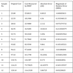
Based on 12 samples, the RREF determines the coefficients that express the contribution of each factor toward the final cost. It is noted that the coefficient of first factor, a1 has a negative value which means it affects on cost reduction when playing alongside with other factors. But literally this cannot be acceptable as each factor is responsible for calculating the total cost, that is the summation of the individual costs. However, it is not irrational to compute the total cost using the generated coefficients for further performance measurement. Now, we put these coefficients in each of 12 equations of type equation (2) to measure the corresponding cost. Table 3 shows the calculated cost for these 12 samples using the proposed first step model and compares with the original cost collected from the AMC.

Table -3: Original AMC Cost vs First Step Model Cost

Sample

No. Original Cost Cost Measured by RREF Absolute Error (AE) Magnitude of Relative Error (MRE)

1 25.80 25.8015 0.0015 -0.00005813

2 22.55 18.1900 4.36 0.193348115

3 28.02 25.9080 2.112 0.075374732

4 46.95 36.9285 10.0215 0.213450479

5 53.74 50.2440 3.496 0.065053964

6 74.13 51.7860 22.344 0.301416431

7 93.82 83.9590 9.861 0.105105521

8 96.61 97.6600 1.05 -0.01086844

9 97.43 43.1798 54.2502 0.556812583

10 134.76 126.587 8.173 0.06064856

11 116.23 73.79025 42.43975 0.365135937

12 120.10 116.2328 3.86725 0.03220025

© 2016, IRJET | Impact Factor value: 4.45 | ISO 9001:2008 Certified Journal | Page 411

found in step one. For this purpose, we formulate this linear system as optimization problem. The aim is to find the coefficients of factors such that the error is minimized close to zero. In this process, 12 observations are taken for the analysis and we use GA solver function in Matlab [23] to find the coefficients subject to minimal errors between total cost and summed individual cost for each factor, expressed as follows-

Min (Error) = Total Cost -

The question is now whether the optimization problem is single objective or multi-objective. We have 5 variables or factors to be considered in the fitness function. 12 observations generate 12 fitness functions for which a set of 5 coefficients are obtained after a particular optimization process. If we consider only one fitness function that means the coefficients are generated only based on 5 factor values for single observation. But we need to determine coefficients in such a way that the errors are minimized for all 12 observations. Therefore, we must take 12 fitness functions into account and hence the problem is a multi-objective optimization problem. So, we can define the fitness function as-

subject to yk = 0, for all k

where k is the number of observations and Ck denotes the total cost for the observation k; akiis the coefficient of i-th factor, xki, in k-th observation.

In Matlab R2010a, we run the fitness function under the GA solver for multi-objective problem. The solver function is expressed as-

gamultiobj (FitnessFunction, numberOfVariables, A, b, Aeq, beq, lb, ub);

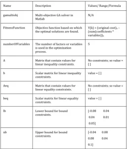
where gamuliobj is the original solver function with eight parameters. Table 4 shows the meaning of the parameters and specifies the values we consider for initial experiment with GA.

It is noted that we take the coefficients from the step one model for creating the lower bound (lb) and upper bound (ub) for which GA can search within the specified boundary close to the obtained coefficients in step one model. For example, the lb = [-0.08 0.04 0.04 0.01 0.05] and the ub = [-0.04 0.08 0.08 [-0.04 0.1] represent that GA looks for coefficient in between -0.08 and -0.04 for the first factor and so on. We name this finding as GAFIRST. Here, the broader the search boundary GA takes more time to find feasible

solutions. At this point, we understand that the negative coefficient for the first factor is not rational, but we aim to obtain such a value that produce better results using GA than produced by RREF. The result informs us whether there is any improvement possible made by GA. Later, we analyze coefficients with a positive range of value for the first factor and vary other factors as well. We repeat the process and performance measurement andname the finding as GASECOND.

Table -4: Matlab Multi-Objective GA Solver Parameters

Name Description Values/ Range/Formula

gamultiobj Multi-objective GA solver in

Matlab

N/A

FitnessFunction Objective function based on which

the optimal solutions are found. Y(k) = (original cost)(sum(coefficients * k – variables))k

numberOfVariables The number of factors or variables is used in the optimization process.

5

A Matrix that contain values for

linear inequality constraints. No constraints; so value = [ ]

b Scalar matrix for linear inequality

constraints. value = [ ]

Aeq Matrix that contain values for

linear equality constraints.

No constraints; so value = [ ]

beq Scalar matrix for linear equality

constraints. value = [ ]

lb Lower bound for bound

constraints.

[-0.08 0.04

0.04 0.01

0.05]

ub Upper bound for bound

constraints. [-0.04 0.08

0.08 0.04

0.1]

6. RESULTS AND DISCUSSION

We complete the standard 30 runs of the GA solver function and we obtain a set of 5 coefficients, 30 times. We pick three better solutions where the error is the best minimized. We tabularize the coefficients obtained by multi-objective GA solver in Table 5 and measure the performance based on the evaluation criteria in Table 6. We also measure few other metrics for better conclusion and understanding for the validity of the model.

Table -5: Coefficient of cost factors obtained in GAPRIMARY

Coefficients a1 a2 a3 a4 a5

© 2016, IRJET | Impact Factor value: 4.45 | ISO 9001:2008 Certified Journal | Page 412

basis of evaluation criteria. Among three best cases the maximum improvement in MAE is occurred by 31.5% against RREF. Based on the other outcomes GAFIRST has MAE = 9.246, MMRE = 0.115 and MAPE = 10.71 %. Therefore, GA performs better than traditional RREF and we are motivated to expand our investigation further.

Table -6: RREF Cost vs GAFIRST Cost vs GASECOND Cost

Metrics Best 1

(GAFIRST)

Best 2

(GAFIRST)

Best 3

(GAFIRST)

Best 1

(GASECOND)

Best 2

(GASECOND)

Best 3

(GASECOND)

a1

-0.0455 -0.0418 -0.0404 0.0165 0.0161 0.0468

a2 0.0566 0.0708 0.0597 0.0677 0.0493 0.0410

a3 0.0563 0.0466 0.0634 0.0471 0.0326 0.0375

a4 0.0119 0.0256 0.0337 0.0193 0.0273 0.0144

a5 0.0988 0.0701 0.0620 0.0212 0.0431 0.0372

Improved in samples (n/12)

9/12 9/12 9/12 9/12 9/12 9/12

Improved MAE (%)

30.468 31.499 30.040 46.251 64.266 54.470

Improved MMRE (%)

61.824 50.958 70.295 98.525 80.130 127.959

Improved MAPE (%)

35.014 35.121 18.275 50.452 64.743 54.545

Maximum deviation among 12 samples

41.021 34.387 36.492 25.325 19.619 16.656

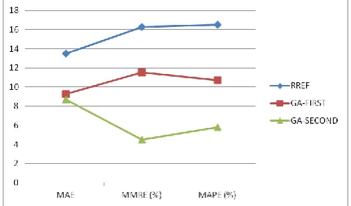
At this stage, we again calibrate the lower and upper parameters with broader range and set a positive range for the first factor to bias the solution within that positive range. The range of values has not taken far away from negative values as it could diverge the solution from the original solution. The parameters are, lb = [0.01 0.03 0.03 0.005 0.02] and the ub = [0.05 0.09 0.09 0.06 0.2]. We repeat the same process for obtaining coefficients using new boundary values that eventually yields more improved measurement. Table 6 displays three best coefficients and compare the performance based on evaluation criteria. Here we obtain far significant outcomes with MAE = 8.679, MMRE = 0.045 and MAPE = 5.78%. From the chart 1 we can easily visualize the performance comparisons of GAFIRST and GASECOND over RREF. We also notice that the improvement has mostly happened in the last column (Best 3 in GASECOND step) in Table 6. If we consider that set of coefficients we obtain measured costs for all 12 samples. Similarly, if we take best coefficients from

GAFIRST we obtain another set of measured costs for all 12

observations. Finally, we compare three step models (RREF,

GAFIRST andGASECOND) in terms of cost measurement against

the original cost. Chart 2 shows the comparisons and we see the GASECOND performs better than other twos in all cases. For example, in sample 9 and 10, measured costs have been deviated downward too much for RREF and GAFIRST where

GASECOND has performed significantly well with more success.

Chart -1: Comparison among RREF, FIRST and GA-SECOND in terms of MAE, MMRE (%) and MAPE (%).

Chart -2: Comparison among RREF, FIRST and GA-SECOND in terms of calculated cost against original cost.

To validate the model, we pick a test case with values of five factors and measure cost using GASECOND. We use SS = 450, SIAS = 455, RRS = 460, IRDTO = 465, and DTO = 470; total cost becomes 81.15 where the original cost is 80.33 from AMC. Using RREF the measured cost is = 76.43. It proves, therefore, our proposed model performs significantly well in every combination of values from AMC.

7. Conclusions

© 2016, IRJET | Impact Factor value: 4.45 | ISO 9001:2008 Certified Journal | Page 413

considering various aspects where they often used Amazon EC2, S3, and Windows Azure as an underlying platform. In this study, we develop a two-step model that identify cost drivers and investigate their behavior over total expense at first step and improve the performance of the overall model by GA at the second step. In AMC, they provide detailed cost for every class of storage but our model provides the contributing effect of each factor that gives an idea of what storage computing class is affecting how much regarding the total cost measurement.

The performance of overall model is significantly well when factors are participated together. An absent of one or more factors can degrade the performance a bit which is yet to be explored. Nevertheless, the performance of the model is noteworthy but can be improved further by taking more samples from the Amazon S3 calculator to produce more accurate estimation. A real time data collection process is useful in this regard as the cost may vary over time. Artificial Neural Network (ANN), a comprehensive machine learning method, can also be investigated for tuning factor coefficients as the data patterns are somewhat non-linear. The similar study can be applied to other related platforms such as Windows Azure, Google Drive etc. and would be worthy to compare results across platforms.

REFERENCES

[1] J. Wu, L. Ping, X. Ge, Y. Wang and J. Fu, “Cloud storage as the infrastructure of cloud computing,” in international conference on intelligent computing and cognitive informatics, 2010, pp. 380-383.

[2] H. Abu-Libdeh and L. Princehouse, “RACS: A Case for Cloud Storage Diversity,” in proceedings of the 1st ACM symposium on Cloud computing, Jun. 10-11, 2010, pp. 229-240, doi: 10.1145/1807128.1807165.

[3] M.R. Palankar, A. Iamnitchi and M. Ripeanu, “Amazon S3 for Science Grids: a Viable Solution?,” in proceedings of the 2008 international workshop on data-aware distributed computing, Jun. 24, 2008, pp. 55-64, doi: 10.1145/1383519.1383526.

[4] E. Walker, "Benchmarking amazon EC2 for hig-performance scientific computing," in the magazine of USENIX & SAGE, vol. 33, Oct. 5, 2008, pp. 18-23. [5] Y. Singh, K. Farah and W. Zhang, "A secured

cost-effective multi-cloud storage in cloud computing," in IEEE conference on computer communications workshops, Apr. 10-15, 2011, pp. 619-624.

[6] S. Garfinkel, "Commodity grid computing with amazon’s s3 and ec2," in The magazine of USENIX, Feb. 2007. [7] E. Deelman, G. Singh, M. Livny andB. Berriman. "The cost

of doing science on the cloud: the montage example," in proceedings of the 2008 ACM/IEEE conference on supercomputing, Nov. 15-21, 2008.

[8] C. Wang, K. Ren, W. Lou and J. Li, "Toward publicly auditable secure cloud data storage services," in IEEE network, vol. 24, 2010, pp. 19-24.

[9] K.D. Bowers, A. Juels, A. Oprea, "HAIL: a high-availability

[10] and integrity layer for cloud storage," in proceedings of the 16th ACM conference on computer and communications security, Nov. 9-13, 2009, pp. 187-198, doi:10.1145/1653662.1653686.

[11] C. Wang, S.S.M. Chow, Q. Wang, K. Ren, "Privacy-preserving public auditing for secure cloud storage," in IEEE transactions on computers, vol. 62, 2013, pp. 362-375.

[12] “Amazon S3 Monthly Calculator,” Available: https://calculator.s3.amazonaws.com/index.html, Aug. 16, 2016.

[13] “Cloud Storage Class – Amazon Simple Storage Services,” Available: https://aws.amazon.com/s3/storage-classes/, Aug. 16, 2016.

[14] “Amazon S3 Reduced Redundancy Storage,” Available: https://aws.amazon.com/s3/reduced-redundancy/, Aug. 16, 2016.

[15] “Cloud Storage Pricing – Amazon Simple Storage Services,”[Online:https://aws.amazon.com/s3/pricing/] , Aug. 16, 2016.

[16] S. J. Leon, “Linear algebra with applications,” (8th

edition), Available:

http://www.academia.edu/download/36340306/Linea r_Algebra_with_Applications_-_8th_-_Leon.pdf, Aug. 05, 2016.

[17] “Linear Algebra / Row Reduction and Echelon Forms,” Available:

https://en.wikibooks.org/wiki/Linear_Algebra/Row_Re duction_and_Echelon_Forms, Aug. 05, 2016.

[18] D. E. Goldberg, “Genetic Algorithms in Search, Optimization and Machine Learning” (1st edition), 1989.

[19] “Genetic Algorithm,” Available:

https://www.mathworks.com/discovery/genetic-algorithm.html, Aug. 13, 2016.

[20] K. Deb, “An efficient constraint handling method for genetic algorithms,” in computer methods in applied mechanics and engineering, vol. 186, 2000, pp. 311-338. [21] Y. Ge and G. Wei, “GA-based task scheduler for the cloud computing systems,” in IEEE international conference on web information systems and mining (WISM), 2010, pp. 181-186.

[22] K. Dasgupta, B. Mandal and P. Dutta, “A genetic algorithm (ga) based load balancing strategy for cloud computing,” in international conference on computational intelligence modeling techniques and applications, 2013, pp. 340-347.

[23] “Reduced Row Echelon Form Calculator,” Available:

http://www.math.odu.edu/~bogacki/cgi-bin/lat.cgi?c=rref, Aug. 7, 2016.

[24] “Performing a Multiobjective Optimization Using the

Genetic Algorithm,” Available:

© 2016, IRJET | Impact Factor value: 4.45 | ISO 9001:2008 Certified Journal | Page 414