Fuzzy Inventory Model for Deteriorating Items with Time Dependent Demand and Partial Backlogging

(1)

http://dx.doi.org/10.4236/am.2015.63047

How to cite this paper: Kumar, S. and Rajput, U.S. (2015) Fuzzy Inventory Model for Deteriorating Items with Time Depen-dent Demand and Partial Backlogging. Applied Mathematics, 6, 496-509. http://dx.doi.org/10.4236/am.2015.63047

Fuzzy Inventory Model for Deteriorating

Items with Time Dependent Demand and

Partial Backlogging

Sushil Kumar

*

, U. S. Rajput

Department of Mathematics & Astronomy, University of Lucknow, Lucknow, India Email: *[email protected]

Received 10 February 2015; accepted 10 March 2015; published 11 March 2015

This work is licensed under the Creative Commons Attribution International License (CC BY). http://creativecommons.org/licenses/by/4.0/

Abstract

In this paper we developed a fuzzy inventory model for deteriorating items with time dependent demand rate. Shortages are allowed and completely backlogged. The backlogging rate of unsatis-fied demand is assumed to be a decreasing exponential function of waiting time. The demand rate, deterioration rate and backlogging rate are assumed as a triangular fuzzy numbers. The purpose of our study is to defuzzify the total profit function by signed distance method and centroid me-thod. Further a numerical example is also given to demonstrate the developed crisp and fuzzy models. A sensitivity analysis is also given to show the effect of change of the parameters.

Keywords

Inventory, Deterioration, Shortages, Triangular Fuzzy Number, Signed Distance Method and Centroid Method

1. Introduction

In many inventory models uncertainty is due to fuzziness and fuzziness is the closed possible approach to reality. In recent years some researchers gave their attention towards a time dependent rate because the demand of newly launched products such as fashionable garments, electronic items, mobiles etc. increases with time and later it becomes constant. Deterioration is defined as damage, decay or spoilage of the items that are stored for future use always loose part of their value with passage of time, so deterioration cannot be avoided in any business

scenarios. F. Harris (1915) [1] developed first inventory model. Lotfi A. Zadeh (1965) [2] introduced the

con-cept of fuzzy set theory in inventory modeling. L. A. Zadeh [3] and R. E. Bellman (1970) considered an

(2)

tory model on decision making in fuzzy environment. R. Jain (1976) [4] developed a fuzzy inventory model on

decision making in the presence of fuzzy variables. D. Dubois and H. Prade (1978) [5] defined some operations

on fuzzy numbers. J. Kacpryzk and P. Staniewski (1982) [6] developed an inventory model for long term

inven-tory policy making through fuzzy decisions. H. J. Zimmerman (1983) [7] tried to use fuzzy sets in operational

research. G. Urgeletti Tinarelli (1983) [8] considered the inventory control models and problems. K. S. Park

(1987) [9] define the fuzzy set theoretical interpretation of an EOQ problem. M. Vujosevic, D. Petrovic and R.

Petrovic (1996) [10] developed an EOQ formula by assuming inventory cost as a fuzzy number. J. S. Yao and H.

M. Lee (1999) [11] developed a fuzzy inventory model by considering backorder as a trapezoidal fuzzy number.

C. K. Kao and W. K. Hsu (2002) [12] developed a single period inventory model with fuzzy demand. C. H.

Hsieh (2002) [13] developed an inventory model and give an approach of optimization of fuzzy production. J. S.

Yao and J. Chiang (2003) [14] developed an inventory model without backorders and defuzzified the fuzzy

holding cost by signed distance and centroid methods. Sujit D. Kumar, P. K. Kund and A. Goswami (2003) [15]

developed an economic production quantity model with fuzzy demand and deterioration rate. J. K. Syed and L.

A. Aziz (2007) [16] consider the signed distance method for a fuzzy inventory model without shortages. P. K.

De and A. Rawat (2011) [17] developed a fuzzy inventory model without shortages by using triangular fuzzy

number. C. K. Jaggi, S. Pareek, A. Sharma and Nidhi (2012) [18] developed a fuzzy inventory model for

deteri-orating items with time varying demand and shortages.

Sumana saha and Tripti Chakrabarty (2012) [19] developed a fuzzy EOQ model with time varying demand

and shortages. D. Dutta and Pawan Kumar (2012) [20] considered a fuzzy inventory model without shortages

using a trapezoidal fuzzy number. D. Dutta and Pawan Kumar (2013) [21] [22] considered an optimal

reple-nishment policy for an inventory model without shortages by assuming fuzziness in demand, holding cost and

ordering cost. Dipak Kumar Jana, Barun Das and Tapan Kumar Roy (2013) [23] give a fuzzy generic algorithm

approach for an inventory model for deteriorating items with backorders under fuzzy inflation and discounting over random planning horizon.

In this paper we consider an inventory model for deteriorating items with time dependent demand rate and partial backlogging. Shortages are allowed and completely backlogged for the next replenishment cycle. The demand rate, deterioration rate and backlogging rate are assumed as triangular fuzzy numbers. The purpose of our study is to defuzzify the total profit function by signed distance method and centroid method and comparing

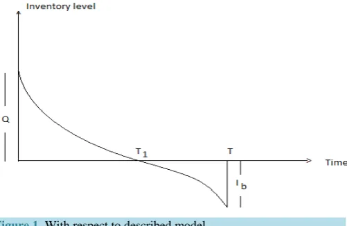
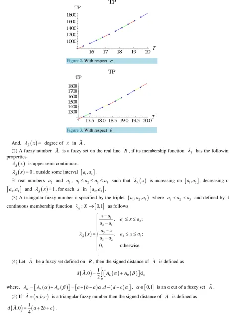
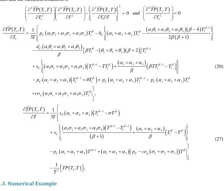
the results of these two methods with the crisp model. Figure 1 shows the developed model and Figure 2 and

Figure 3 show the graphs of total profit function with respect to deterioration and backlogging rates.

2. Definitions and Preliminaries

When we are considering the fuzzy inventory model then the following definitions are needed.

(1) A fuzzy set A on the given universal set X is denoted and defined by

( )

(

)

{

, :

}

A

A= xλ_ x x∈X

[image:2.595.173.424.553.716.2]

where, λ_A:X →

[ ]

0,1 , is called the membership function,

(3)

[image:3.595.73.535.86.728.2]

Figure 2. With respect σ.

Figure 3. With respect θ.

And,

( )

A x

λ_ = degree of x in A .

(2) A fuzzy number A is a fuzzy set on the real line R, if its membership function

λ

_A_ has the following

properties

( )

A x

λ_ is upper semi continuous.

( )

0 A x

λ_ = , outside some interval

[

a a₁, ₄

]

.

∃ real numbers a₂ and a₃, a₁≤a₂≤a₃≤a₄ such that λ_A

( )

x is increasing on

[

a a1, 2

]

, decreasing on

[

a a3, 4

]

and λA

( )

x =1, for each x in

[

a a2, 3

]

.

(3) A triangular fuzzy number is specified by the triplet

(

a a a₁, ₂, ₃

)

where a₁a₂a₃ and defined by its

continuous membership function λ_A:X →

[ ]

0,1 as follows

( )

1

1 2

2 1

3

2 3

3 2

, ;

0, otherwise. A

x a

a x a a a

a x

x a x a

a a

λ

−

 _{≤ ≤}

 − 

 −

=_ ≤ ≤

−    



(4) Let A be a fuzzy set defined on R, then the signed distance of A is defined as

( )

1

( )

0

1

, 0 d

2 L R

d A =

∫

A α +A β  α

where, A_α =_A_L

( )

α +A_R

( )

β _{ } = a+

(

b−a

)

α,d−

(

d−c

)

α_, α ∈

[ ]

0,1 is an α cut of a fuzzy set A .

(5) If A=

(

a b c, ,

)

is a triangular fuzzy number then the signed distance of A is defined as

( )

1

(

)

, 0 2

4

d A = a+ b+c .

16 17 18 19 20 T

1000 1200 1400 1600 1800

TP

17.5 18.0 18.5 19.0 19.5 20.0T 1300

1400 1500 1600 1700 1800 TP

(4)

(6) If A=

(

a b c, ,

)

is a triangular fuzzy number then the centroid method on A is defined as

( )

1

(

)

3

C A = a b c+ + .

3. Assumptions and Notations

We consider the following assumptions and notations.

The demand rate is R t

( )

=αtβ−1 where α is a positive constant, for a increasing demand β >1, and for a

decreasing demand β<1.

1. θ is the deterioration parameter.

2. σ is the backlogging parameter.

3. A is the ordering cost per order.

4. h_c is the holding cost per unit per unit time.

5. d_c is the deterioration cost per unit per unit time.

6. s_c is the shortages cost per unit per unit time.

7. p_c is the purchase cost per unit.

8. s_p is the selling price per unit, where s_p p_C.

9. opC is the opportunity cost per unit due to lost sales.

10.T is the length of order cycle.

11.θ is the fuzzy deterioration parameter.

12.σ is the fuzzy backlogging parameter.

13.α is the fuzzy demand parameter.

14.TP T T

(

₁,

)

is the total fuzzy profit per unit time.

15.T₁ is the time at which shortage starts.

16.TP T T

(

₁,

)

is the total profit per unit time.

17.I t

( )

is the inventory level at any time in

[ ]

0,T .

18.The inventory system consists only one item.

19.The time horizon T is infinite.

20.The lead time is zero.

21.The replenishment rate is infinite.

3.1. Mathematical Formulation

Suppose an inventory system consists Q units of the product in the beginning of each cycle. Due to demand

and deterioration the inventory level decreases in

[

0,T₁

]

and becomes zero at t=T₁. The interval

[

T T₁,

]

is

the shortages interval. During the shortages interval the unsatisfied demand is backlogged at a rate of e−σt,

where t is the waiting time.

The instantaneous inventory level at any time t in

[

0,T₁

]

are governed by the following differential

equa-tions

1

d

, 0 d

I

I t t T

t

β

θ α −

+ = − ≤ ≤ (1)

with boundary condition I

( )

0 =Q

1

d

e , d

t

I

t T t T

t

β σ

α − −

= − ≤ ≤ (2)

with boundary condition I T

( )

₁ =0

( )

e

₍

1

_{) (}

2

₎

2

1 1

t t t t

I t Q

β β β

θ α αθ αθ

β β β β

+ +

−

= − + +

(5)

The solution of Equation (1) is

( )

(

) (

)

(

) (

)

1

1 2 2 1 2 2

1 1 1

e

1 1 1 1

T t T T T t t t

I t

β β β β β β

θ α αθ αθ α αθ αθ

β β β β β β β β

+ + + +

−  

= _ − − _− + +

+ + + +

 

  (4)

The solution of Equation (2) is

( )

(

1 1

) (

)

1 1

1

I t ασ tβ Tβ α Tβ tβ

β β

+ +

= − + −

+ (5)

using I T

( )

₁ =0, in Equation (3)

(

) (

)

1

1 2 2

1 1 1

e

1 1

T T T T

Q

β β β

θ α αθ αθ

β β β β

+ +

 

 

=  − ₊ − ₊ 

 

  (6)

The ordering cost per cycle is

C

O =A (7)

The holding cost per cycle is

( )

(

)(

)

(

)

1

0

1 2 2 3

1 1 1

d ;

1 1 1 1 1

1 .

1 2 1 1 2 1 2 3

T

C C

H h I t t

T T T

H h

β β β

α αθ αθ

+ + +

=

    

=  ₊ +  − ₊ + ₊ ₊ − ₊  + − ₊ 

   

   

 

∫

(8)

The deterioration cost per cycle is

1

0

1 2 2

1 1

d ;

. 1

T

C C

D d Q t t

T T

D d

β

β β

α

αθ αθ

β β

−

+ +

 

=  − 

 

 

 

= _ − _

+

 

∫

(9)

The shortage cost per cycle is

( )

(

)

(

)

1

2 1

1 1 1

1 1

d ;

1

.

1 2 2 1 1

T

C C

T

C C

S s I t t

T T

S s TT TT

β β β

β β

β

ασ α

β β β β β β

+ + +

+

= −

  +   

=  ₊  ₊ + ₊ − +  − ₊ − ₊ 

 

    

 

∫

(10)

The purchase cost per cycle in

[

0,T₁

]

is

1

1 2 2

1 1 1

1

;

. 1

C

PC p Q

T T T

PC p

β β β

α αθ αθ

β β β

+ +

=

 

= _ + − _

+

 

(11)

The purchase cost per cycle in

[

T T₁,

]

is

(

)

(

)

(

)

1

1 2

2

1 1

2 1 1

e d ;

. 1

C

C C

T

t

T

PC p t t

p p

PC T T T T

β σ

β β β β

α

α α

β β

− −

+ +

=

= − − −

+

∫

(12)

(6)

(

)

(

)

1 1 1 1 1 1

e d ;

. 1 T t p p T p p

CO co t t t

co

CO T T

β β σ

β β α α ασ β − − − + + = − = − +

∫

(13)

The sales revenue cost per cycle in

[ ]

0,T is

(

)

1 1 1 1 0 1 1 1

d e d ;

. 1 1 T T t R R T R R

S s t t t t

T

T T

S s

β β σ

β

β β

α α

ασ

α ασ

β β β

− − − + +   =  +        = _ − + _ + +  

∫

(14)

Therefore the total profit per unit time is

(

)

[

]

(

)

(

)(

)

(

)

1 1 2

1 1

1 2 2 3

1 1 1

1

, ;

1 ,

1 1

1 1 1 1 1

1

1 2 1 1 2 1 2 3

R C C C C P

R

C

TP T T S O H D S PC PC CO

T

T T

TP T T s A

T

T T T

h

d

β

β β

β β β

ασ

α ασ

β β β

α αθ αθ

α + + + + + = − − − − − − −    = _{ } − + − + +            −  ₊ + _ − ₊ + ₊ ₊ _− ₊  + − ₊          −

(

)

(

)

(

)

(

)

2

1 2 2 2 1 1

1 1

1 1 1

1 1

2

1 2 2

1 1

1 1 1

1 1

1

1 1 2 2 1 1

1 1 C C C C T

T T T T T

s TT TT

p p

T T T

p T T T T

β

β β β β β

β β

β β β

β β β β

β

θ αθ ασ α

α α

α αθ αθ

β β β β β

+ + + + + + + + + + +   +    ₋ ₊  ₊ ₋ ₊  ₋ ₋     ₊   ₊ _ ₊ ₊ _  ₊ ₊           −  + ₊ − − − + ₊ −  

(

1 1

)

1

. 1

p

co

Tβ Tβ

ασ β + +  − − _ + _ (15)

For a Ist order approximation of e−θt

(

)

₍

₎

(

)

(

)

1

1 1 2

1

1 1 1

1

2 1

1 1 1

1 1

1

, [

1 1 1 2 2 1

1

1 2 2 1 1

C

R C

C

d T

T T T

T T

TP T T s A h

T

T T

s TT TT

β

β β β

β β

αθ

ασ α αθ

α ασ

β β β β β β

β

ασ α

β β β β β β

+ + + + + + + + + +     _ _ = _ − + _− − _ + _− + + _ + + _ +       +      +  ₊ _ ₊ + ₊ − _+  − ₊ − ₊         

(

)

(

)

(

)

1 1 1 1 1 1 1 1 1 1 1 1 , 1 C C C p p p T T

p T T T T

co

T T

β β

β β β β

β β

α α

α αθ

β β β β

ασ β + + + + +   − _ + _− − + − + +    − − _ + _ (16)

The necessary condition for TP T T

(

₁,

)

to be maximum is that

(

1

)

1

, 0

TP T T T

∂

=

∂ and

(

1,

)

0 TP T T

T

∂

=

∂ , and

solving these equations we find the optimum values of T₁ and T say T₁∗ and T∗ for which profit is maxi-

mum and the sufficient condition is

(

)

(

)

(

)

2

2 2 2

1 1 1

2 2

1 1

, , ,

0

TP T T TP T T TP T T T T

T T

∂ ∂  ₋∂ 

    

 _∂  _∂  _ _{∂ ∂} _

      and

(

)

2 1 2 1 , 0 TP T T

T

∂ 

 

 _∂ 

(7)

(

)

(

)

(

)

{

(

)

}

(

) (

)

(

)

1

1 1 1

1 1 1 1

1

1 1 1 1

1 1 1 1 1 1 1

1 1

, 1 4

2 2 1 C C C

C C C

C p

TP T T T d

p T h T T T

T T

s T TT TT T p T T p T

p T co T

β

β β β β

β β β β β β β

β β

αθ β αθ

ασ α β θ β

β β β

α

σα β α θ α

β α ασ + + + − − −    ∂ ₌ ₋  ₋ − ₋ ₋ ₊    ∂ __ __ + __   +  − + − − + +    − + _ , (17)

(

)

₍

₎

(

)

(

)

(

)

(

)

(

)

1 1 1

1 1 1 2 , 1 1 1 , ,

P C C C p

T T

TP T T

s T T s T T p T p co T

T T

TP T T T

β β

β β ασ α β β β β

α σ α α σ

β β + + − +   −   ∂ _ _ _ _ = − + _ + − _− + −   ∂ __ + __   − _ _ (18)

3.2. Fuzzy Model

Let us consider the inventory model in fuzzy environment due to uncertainty in parameters let us assume that the

parameters θ, α and σ may change within some limits.

Let θ=

(

θ θ θ₁, ₂, ₃

)

, α =

(

α α α₁, ₂, ₃

)

and σ =

(

σ σ σ₁, ₂, ₃

)

are triangular fuzzy numbers then the total prof-it per unprof-it time in fuzzy sense is



₍

₎

(

)

(

)

(

)

1

1 1 2

1

1 1 1

1

2 1

1 1 1

1 1

1 ,

1 1 1 2 2 1

1

1 2 2 1 1

C

R C

C

d T

T T T

T T

TP T T s A h

T

T T

s TT TT

β

β β β

β β

αθ

ασ α αθ

α ασ

β β β β β β

β

ασ α

β β β β β β

+ + + + + + + + + +    _ _ = _{ } − + _− − _ + _− + + _ + + _ +        +    + ₊ _ ₊ + ₊ − _+  − ₊ − ₊       _        

(

)

(

)

(

)

1

1 1 1 1

1 1

1 1 1

,

1 1 1

p C C C co p p T T

p T T T T T T

β β

β β β β ασ β β

α α

α αθ

β β β β β

+ + + + +                −  + ₊ − − + ₊ − − ₊ −               (19)

Now we defuzzify the total profit TP T T

(

₁,

)

in two cases.

3.2.1. Signed Distance Method

By signed distance method the total profit per unit time is



₍

₁

₎

1

₍

₁

₎

2

₍

₁

₎

3

₍

₁

₎

1

, , 2 , ,

4

TP T T TP T T TP T T TP T T

T  

= _ + + _ (20)

where,



₍

₎

(

)

(

)

(

)

1 1 1 2

1 1 1 1 1 1 1 1 1 1 1

1 ₁

2 1

1 1

1 1 1 1

1 1

1 ,

4 1 1 1 2 2

1

1 2 2 1 1

R C

C

T T T T T

TP T T s A h

T

T T

s TT TT

β β β β β

β β

α α σ α σ α α θ

β β β β β

β

α σ α

β β β β β β

+ + + + + + + + +      = _{ } − ₊ + ₊ − −  ₊ + ₊            +    + _ + − _+  − −  + _ + + _ _ + + _           

(

)

(

)

(

)

1 1 1 1 1

1 1

1

1 1 1 1

1 1 1

1 1 1 , 1 1 C C C p C p p T T

p T T T T

co d T

T T

β β

β β β β

β

β β

α α

α α θ

β β β β

(8)



₍

₎

(

)

(

)

(

)

1 1 1 2

2 2 2 2 2 1 2 1 2 2 1

2 ₁

2 1

1 1

2 2 2 1

1 1

1 ,

4 1 1 1 2 2

1

1 2 2 1 1

R C

C

T T T T T

TP T T s A h

T

T T

s TT TT

β β β β β

β β

β β β β β

β

α σ α

β β β β β β

+ + + + + + + + +      = _{ } − ₊ + ₊ − −  ₊ + ₊            +    + ₊ _ ₊ + ₊ − _+  − ₊ − ₊                

(

)

(

)

(

)

1 1 1 2 2

2 1 2 2 1

1 1

1

2 2 1 1

2 2 1

1 1 1 , 1 1 C C C p C p p T T

p T T T T

co d T

T T

β β

β β β β

β

β β

α α

α α θ

β β β β

α σ α θ β β + + + + + +              − _ + _− − + − + +      − − − _ + + _  _ _       

₍

₎

(

)

(

)

(

)

1 1 1 2

3 3 3 3 3 1 3 1 3 3 1

3 ₁

2 1

1 1

3 3 3 1

1 1

1 ,

4 1 1 1 2 2

1

1 2 2 1 1

R C

C

T T T T T

TP T T s A h

T

T T

s TT TT

β β β β β

β β

β β β β β

β

α σ α

β β β β β β

+ + + + + + + + +  _ _ _ _ = _{ } − + _− − _ + _ + + + +            +   + ₊ _ ₊ + ₊ − _+  − ₊ − ₊              

(

)

(

)

(

)

1 1 1

3 1 3 3 1 3 3

1 1

1

3 3 1 1

3 3 1

1 1 1 , 1 1 C C C p C

T T p p

p T T T T

co d T

T T

β β

β β β β

β

β β

α α θ α α

β β β β

α σ α θ β β + + + + + +                − _ + _− − + − + +      − − − _ + + _         

From Equation (20) we have



₍

₎

(

)

(

)

(

)

(

)

(

)

(

)

(

)

(

)

1 1 1

1 2 3 1 1 2 2 3 3 1 1 2 2 3 3 1

1 2

1 2 3 1 1 1 2 2 3 3 1

2 2

1 1 2 2 3 3 1

,

2 2 2

1

4

4 1 1

2 2

1 2 2

2 1 1 2 R C C

TP T T

T T T

s A T T T h T T s

β β β

β β

α α α α σ α σ α σ α σ α σ α σ

β β β

α α α α θ α θ α θ

β β

α σ α σ α σ β

β β β

+ + + + + +   + + + + + +  = _{ } − + _− + +      + + + +    −  +  + +     + + + + + + +

(

+

)

(

)

(

)

(

)

(

)

₍

₎

(

)

(

)

1 1

1 2 3

1 1

1

1 2 3 1 1 1 2 2 3 3 1

1 2 3 1 2 3 1 1

1 1

1 1 2 2 3 3

2

2 1 1

2 2 1 2 2 ( ) 1 2 C C C T T TT TT T T p p p

T T T T

β β

β β β β

α α α

β β β

β β

α α α α α α

β β

α θ α θ α θ

+ + + + + +    + +    ₋ ₊ ₋ ₋     _ _   + +          + + + +    − _ + _ +     + + + + − − + − + + + −

(

)

(

)

1

1 1 2 2 3 3

1 1 1

1 2 . 1 1 p C co d T T T β β β

α σ α σ α σ

β β + + +  + + − −  + + _ (21)

The necessary condition for TP T T

(

₁,

)

to be maximum is that 

(

1

)

1

, 0

TP T T T

∂

=

∂ and



₍

₎

1,

0

TP T T T

∂

=

∂ , and

solving these equations we find the optimum values of T₁ and T say T₁∗ and T∗ for which profit is

maxi-mum and the sufficient condition is



₍

₎



₍

₎



₍

₎

2

2 2 2

1 1 1

2 2

1 1

, , ,

0

TP T T TP T T TP T T T T T T ∂ ∂  _∂ _ −       _∂  _∂  _ _{∂ ∂} _

      and



₍

₎

2 1 2 1 , 0 TP T T

T

∂ 

 

 _∂ 

(9)



₍

₎

(

)

(

)

(

₍

)(

₎

)

(

)

_{

₍

₎₍

₎

_}

(

)

1

1 1 2 2 3 3 1

1

1 1 2 2 3 3 1

1 2 3 1

1 1 2 2 3 3 1

1 1 2 3 1

1

1 1 2 2 3 3 1 1

, 1 2 4 2 4 2 2 1 2 2 2 2 C C C C

TP T T

p T T T T h T d T T

s T TT

β

β β

β

α σ α σ α σ

α θ α θ α θ β

α α α

β β α θ α θ α θ

β θ θ θ β

β

α σ α σ α σ

+ + + ∂  = _ + + ∂  + + −    −  + + − ₊      + + − − + + + + + +

(

−

)

(

)

(

)

(

)

(

)

(

)

(

)

(

)

1 2 3 1

1 1

1 2 3 1 1 1 2 3 1 1 2 3 1

1 1 2 2 3 3 1

2

2 2 2

2 ,

C C C

p

TT T

p T T p T p T

co T

β β β

β β β β

β

α α α

β β

α α α θ α α α α α α

α σ α σ α σ

− − −  + +   ₊ ₋        − + + + + + + − + +  + + + _  (22) 

₍

₎

(

)

(

)

(

)

(

)

(

)

(

)

(

)

(

)

(

)

(

)

(

)

1 1

1 2 3 1

1 1

1 1 2 2 3 3 1 1 2 3

1

1 2 3 1 2 3 1 2 3

1 2 , 1 2 4 2 2 1

2 2 2

1

, P

C

C C p

TP T T

s T T

T T

s T T

p T p co T

TP T T T

β β

α α α σ

α σ α σ α σ α α α

β β

α α α α α α σ σ σ

− + + −  ∂ _ = + + − ∂ _  + + − + +    +  ₊ + −        − + + + + + − + +  − _ _, (23)

3.2.2. Centroid Method

By Centroid method the total profit per unit time is



₍

₁

₎

1

₍

₁

₎

2

₍

₁

₎

3

₍

₁

₎

1

, , , ,

3

TP T T TP T T TP T T TP T T

T  

= _ + + _ (24)



₍

₎

(

)

(

)

(

)

(

)

(

)

(

)

(

)

(

)

(

)

1 1 1

1 2 3 1 1 2 2 3 3 1 1 2 2 3 3 1

1 2

1 2 3 1 1 1 2 2 3 3 1

2 2

1 1 2 2 3 3 1 1

1

, 1

3

3 1 1

1 2 2

1

1 2 2

R

C

TP T T

T T T

s A T T T h T T s TT

β β β

β β

β

α α α α σ α σ α σ α σ α σ α σ

β β β

β β

α σ α σ α σ β

β β β

+ + + + + + +   + + + + + +  = _{ } − + _− + +  _ _   + + + +    − _ + _ + +      + + + + + − + _ + +

(

)

(

)

(

)

(

)

₍

₎

(

)

₍

₎

(

)

1 1

1 2 3 1

1

1 2 3 1 1 1 2 2 3 3 1

1 2 3 1 2 3 1 1

1 1

1

1 1 2 2

1 1 2 2 3 3 1

1 1 1 1 1 C C C p C T T TT T T p p p

T T T T

co d T

β β

β

β β

β β β β

β

α α α

β β β

β β

α α α α α α

β β

α σ α σ α θ α θ α θ

β + + + + + +   + +    ₊ ₋ ₋     _ _  ₊ ₊          + + + +    −  + ₊      + + + + − − + − + + + + + − − +

(

3 3

)

₍

1 1

₎

1 ,

1 T T

(10)

The necessary condition for TP T T

(

₁,

)

to be maximum is that 

(

1

)

1

, 0

TP T T T

∂

=

∂ and



₍

₎

1,

0

TP T T T

∂

=

∂ , and

solving these equations we find the optimum values of T₁ and T say T₁∗ and T∗ for which profit is

maxi-mum and the sufficient condition is



₍

₎



₍

₎



₍

₎

2

2 2 2

1 1 1

2 2

1 1

, , ,

0

TP T T TP T T TP T T T T

T T

∂ ∂  ₋∂ 

    

 _∂  _∂  _ _{∂ ∂} _

     

and 

(

)

2 1 2 1

, 0 TP T T

T

∂ 

 

 _∂ 

 



₍

₎

(

)

(

)

(

₍

)(

₎

)

(

)

_{

₍

₎₍

₎

_}

(

)

1

1 1 2 2 3 3 1

1

1 1 2 2 3 3 1 1 2 3 1

1

1 1 2 2 3 3 1

1 1 2 3 1

1

1 1 2 2 3 3 1 1

4

, 1

3 2 1

2

C C

C

T TP T T

p T h T

T T

d

T T

s T TT

β

β β

β

α θ α θ α θ β

β β α θ α θ α θ

β θ θ θ β

β

α σ α σ α σ

+

  + + − 

∂ ₌ ₊ ₊ ₋  ₊ ₊ ₋ 

  

∂ __ __ + __

+ +

− − + + +

+ + +

(

−

)

(

)

(

)

(

)

(

)

(

)

(

)

(

)

1 2 3 1

1 1

1 2 3 1 1 1 2 3 1 1 2 3 1

1 1 2 2 3 3 1

,

C C C

p

TT T

p T T p T p T

co T

β β β

β β β β

β

α α α

β β

α α α θ α α α α α α

α σ α σ α σ

−

− −

 + + 

 ₊ ₋ 

 

 

 

− + + + + + + − + +



+ + + _



(26)



₍

₎

(

)

(

)

(

)

(

)

(

)

(

)

(

)

(

)

(

)

(

)

(

)

1 1

1 2 3 1

1 1

1 1 2 2 3 3 1 1 2 3

1

1 2 3 1 2 3 1 2 3

1 2

, 1

3

1

, , P

C

C C p

TP T T

s T T

T T

s T T

p T p co T

TP T T T

β β

α α α σ

β β

α α α α α α σ σ σ

−

+ +

−

 ∂



= + + −

∂ _

 + + − ₊ ₊ 

 

+  + − 

+

 

 



− + + + + + − + + 



− _ _

(27)

3.3. Numerical Example

Let us consider an inventory system with the following parameters in appropriate units as Rs200/order

A= s_p =Rs20/unit/year, co_p =Rs6/unit/year, σ =Rs3/unit/year,

8 unit/year

[image:10.595.92.540.137.518.2]

α = , β =1 unit/year

,

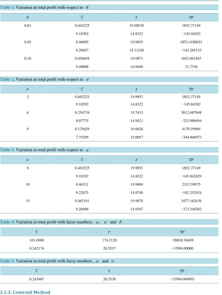
θ =0.01/year

.

Table 1 shows that as we increase deterioration parameter θ then the total profit increases. Table 2 shows that as we increase backlogging parameter σ then the total profit increases. Table 3 shows that as we increase demand parameter α then the total profit increases. 3.3.1. Fuzzy Model

Let α =

(

5,10, 20

)

, σ =

(

3,8,15

)

and θ =

(

0.001, 0.005, 0.150

)

are triangular fuzzy numbers. The solution of the fuzzy inventory model can be determined by the following two methods. 3.3.2. Signed Distance Method

When α, σ and θ are triangular fuzzy numbers, then Table 4 shows the value of total profit.

When α and σ are triangular fuzzy numbers, then Table 5 shows the value of total profit.

(11)

[image:11.595.87.546.76.685.2]

Table 1. Variation in total profit with respect to θ.

θ T1 T TP

0.01 0.463225 19.98530 1852.37149

9.18392 14.8322 −145.84282

0.05 0.46005 19.9855 1852.4180031

9.20047 15.11240 −143.265133

0.10 0.456658 19.9873 1852.861567

9.48808 16.9640 31.7336

Table 2. Variation in total profit with respect to σ.

σ T1 T TP

3 0.463225 19.9853 1852.37149

9.18392 14.8322 −145.84282

6 0.254734 19.7433 3012.687848

8.07775 14.9421 −223.098494

9 0.175629 19.6626 4179.59984

7.75299 15.0057 −344.806973

Table 3. Variation in total profit with respect to α.

α T1 T TP

8 0.463225 19.9853 1852.37149

9.18392 14.8322 −145.842829

10 0.46321 19.9869 2312.59975

9.22675 14.8740 −182.252924

15 0.463191 19.9870 3477.162439

9.28496 14.9307 −273.348202

Table 4. Variation in total profit with fuzzy numbers, α, σ and θ.

1

T T TP

161.6960 174.2120 −38818.36498

0.242176 20.3537 −13994.00000

Table 5. Variation in total profit with fuzzy numbers, α and σ.

1

T T TP

0.243607 20.3538 −13994.069903

3.3.3. Centroid Method

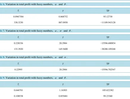
When α, σ and θ are triangular fuzzy numbers, then Table 7 shows the value of total profit.

When α and σ are triangular fuzzy numbers, then Table 8 shows the value of total profit.

(12)

[image:12.595.101.538.77.411.2]

Table 6. Variation in total profit with fuzzy numbers, α and θ.

1

T T TP

0.0967304 0.868752 95.12730

338.3230 887.0950 −11109.943128

Table 7. Variation in total profit with fuzzy numbers, α, σ and θ.

1

T T TP

0.228336 20.2984 −15596.680854

133.3920 145.9400 −38288.109268

Table 8. Variation in total profit with fuzzy numbers, α and σ.

1

T T TP

0.22995 20.2984 −15596.702547

Table 9. Variation in total profit with fuzzy numbers, α and θ.

1

T T TP

0.646701 1.16303 105.622382

0.108538 0.855681 99.23360

4. Sensitivity Analysis

From Table 1, we see that as we increase the deterioration parameter θ then the optimal time period T₁, the

optimal cycle time T and total profit increases.

From Table 2, we see that as we increase the backlogging parameter σ then the optimal time period T₁, the

optimal cycle time T decreases and total profit increases.

From Table 3, we see that as we increase the demand rate parameter α then the optimal time period T₁

decreases and the optimal cycle time T and total profit increases.

In the case of crisp model we see that the backlogging parameter σ is more sensitive than the deterioration

parameter θ and the demand rate parameter α.

From the tables for signed distance method and centroid method we see that the fuzzy variables θ_and α

are more sensitive than the fuzzy variable σ . As we increase the fuzzy variables θ_and α in the signed

distance method and centroid method than the total profit increases rapidly in centroid method. Therefore in the sense of fuzziness the centroid method is better one than the signed distance method.

5. Conclusion

In this paper we studied a fuzzy inventory model for deteriorating items with time dependent demand rate and

partial backlogging. Shortages are allowed and completely backlogged. As we increase the parameters α, σ

and θ in the crisp model then the total profit increases and due to the uncertainties in the demand rate,

deteri-oration rate and backlogging rate the parameters α , σ and θ are consider as triangular fuzzy numbers. For

(13)

Acknowledgements

The author would like to thank anonymous referees for their valuable comments and suggestions for the im-provement of this paper.

References

[1] Harris, F. (1915) Operations and Cost. AW Shaw CO., Chicago.

[2] Zadeh, L.A. (1965) Fuzzy Set. Information Control, 8, 338-353. http://dx.doi.org/10.1016/S0019-9958(65)90241-X

[3] Zadeh, L.A. and Bellman, R.E. (1970) Decision Making in a Fuzzy Environment. Management Science, 17, 140-164.

[4] Jain, R. (1976) Decision Making in the Presence of Fuzzy Variables. IIIE Transactions on Systems, Man and Cyber-netics, 17, 698-703.

[5] Dubois, D. and Prade, H. (1978) Operations on Fuzzy Numbers. International Journal of System Science, 9, 613-626. http://dx.doi.org/10.1080/00207727808941724

[6] Kacpryzk, J. and Staniewski, P. (1982) Long Term Inventory Policy Making through Fuzzy Decision Making Methods.

Fuzzy Sets and System, 8, 117-132. http://dx.doi.org/10.1016/0165-0114(82)90002-1

[7] Zimmerman, H.J. (1983) Using Fuzzy Sets in Operational Research. European Journal of Operation Research, 13, 201-206. http://dx.doi.org/10.1016/0377-2217(83)90048-6

[8] Urgeletti Tinarelli, G. (1983) Inventory Control Models and Problems. European Journal of Operation Research, 14, 1-12. http://dx.doi.org/10.1016/0377-2217(83)90283-7

[9] Park, K.S. (1987) Fuzzy Set Theoretical Interpretation of Economic Order Quantity. IEEE Transactions on Systems,

Man and Cybernetics, 17, 1082-1084. http://dx.doi.org/10.1109/TSMC.1987.6499320

[10] Vujosevic, M. and Petrovic, D. (1996) EOQ Formula When Inventory Cost Is Fuzzy. International Journal of Produc-tion Economics, 45, 499-504. http://dx.doi.org/10.1016/0925-5273(95)00149-2

[11] Yao, J.S. and Lee, H.M. (1999) Fuzzy Inventory with or without Backorder for Fuzzy Order Quantity with Trapezoidal Fuzzy Number. Fuzzy Sets and Systems, 105, 311-337. http://dx.doi.org/10.1016/S0165-0114(97)00251-0

[12] Yao, J.S. and Lee, H.M. (1999) Economic Order Quantity in Fuzzy Sense for Inventory without Backorder Model.

Fuzzy Sets and Systems, 105, 13-31.

[13] Kao, C.K. and Hsu, W.K. (2002) A Single Period Inventory Model with Fuzzy Demand. Computers and Mathematics with Applications, 43, 841-848. http://dx.doi.org/10.1016/S0898-1221(01)00325-X

[14] Hsieh, C.H. (2002) Optimization of Fuzzy Production Inventory Models. Information Sciences, 146, 29-40. http://dx.doi.org/10.1016/S0020-0255(02)00212-8

[15] Yao, J.S. and Chiang, J. (2003) Inventory without Backorder with Fuzzy Total Cost and Fuzzy Storing Cost Defuzzi-fied by Centroid and Signed Distance. European Journal of Operational Research, 148, 401-409.

http://dx.doi.org/10.1016/S0377-2217(02)00427-7

[16] Kumar, Sujit De, Kundu, P.K. and Goswami, A. (2007) An Economic Production Quantity Inventory Model Involving Fuzzy Demand Rate and Fuzzy Deterioration Rate. Journal of Applied Mathematics and Computing, 12, 251-260. http://dx.doi.org/10.1007/BF02936197

[17] Syed, J.K. and Aziz, L.A. (2007) Fuzzy Inventory Model without Shortages by Using Signed Distance Method. Ap-plied Mathematics and Information Sciences, 1, 203-209.

[18] De, P.K. and Rawat, A. (2011) A Fuzzy Inventory Model without Shortages Using Triangular Fuzzy Number. Fuzzy Information and Engineering, 3, 59-68. http://dx.doi.org/10.1007/s12543-011-0066-9

[19] Jaggi, C.K., Pareek, S., Sharma, A. and Nidhi (2012) Fuzzy Inventory Model for Deteriorating Items with Time Vary-ing Demand and Shortages. American Journal of Operational Research, 2, 81-92.

http://dx.doi.org/10.5923/j.ajor.20120206.01

[20] Saha, S. and Chakrabarti, T. (2012) Fuzzy EOQ Model with Time Dependent Demand and Deterioration with Short-ages. IOSR Journal of Mathematics, 2, 46-54.

[21] Dutta, D. and Kumar, P. (2012) Fuzzy Inventory Model without Shortage Using Trapezoidal Fuzzy Numberwith Sen-sitivity Analysis. IOSR Journal of Mathematics, 4, 32-37.

(14)