Study of Surface Soliton at the Interface Between a Semidiscrete One Dimensional Kerr Nonlinear System and a Continuous Medium (Slab Waveguide)

(1)

Study of surface Soliton at the interface between a semidiscrete

one-dimensional Kerr-nonlinear system and a continuous medium

(slab waveguide)

O. P. Swami

1

_{, Vijendra Kumar}

2

_{, A. K. Nagar}

3

1,2,3

_{Department of Physics, Govt. Dungar college, Bikaner, Rajasthan, India, 334001}

---*---Abstract –**

In this paper, we study the existence of Surface Soliton at the interface between a semidiscrete one dimension Kerr-nonlinear system and a continuous medium in form of optical waveguide. We investigate that a power threshold is required for the existence of surface. Below which no excitation found. Power threshold is calculated numerically and analytically with the function of propagation constant (keeping fix value of coupling constant). We also found that increasing the strength of coupling constant between the waveguides increases the light intensity in the excited waveguide resulting in a smoother soliton.

Key Words: Surface Soliton, Waveguides, Discrete nonlinear Schrodinger equation, Kerr-nonlinear system, Refractive index.

1. INTRODUCTION AND REVIEW OF SOME

PREVIOUS WORK

The presence of an interface between different materials can profoundly affect the evolution of nonlinear excitations. Such interface can support stationary surface waves. These were encountered in various areas of physics including solid-state physics [1], near surface optics [2], plasmas [3], and acoustics [4]. In nonlinear optics, surface waves were under active consideration since 1980. The progress in their experimental observation was severely limited because of unrealistically high power levels required for surface wave excitation at the interfaces of natural materials. However, shallow refractive index modulations accessible in a technologically fabricated waveguide array (or lattice) may facilitate the formation of surface waves at moderate power levels at the edge of semi-infinite arrays as was suggested in Ref. [5]. This has led to the observation of one-dimensional surface solitons in arrays with focusing nonlinearity [6]. Defocusing lattice interfaces are also capable to support surface gap solitons [7, 8 & 9]. Surface lattice solitons may exist not only in cubic and saturable materials, but also in quadratic [10] and nonlocal [11] media, as well as at the interfaces of complex arrays [12].

The femtosecond laser direct writing technique [13] allows fabrication of waveguide arrays along arbitrary paths [14] and with various topologies, such as square [15], hexagonal [16] and circular [17], where multiple waveguides

can be specifically excited [18]. Since the nonlinearity of the waveguides is affected by the writing parameters [19], it is possible to tune it for specific purposes, such as excitation of 1D and 2D discrete solitons [20 & 21].

Surface solitons have also been predicted at the interface between two different semi-infinite waveguide arrays [22], as well as at the boundaries of two-dimensional (2D) nonlinear lattices [23, 24, 25, 26 & 27]. It has been shown that surface solitons of the vectorial [28 & 29] and vertical [6.77] types, as well as surface kinks [30], can exist too.

The existence of surface Soliton required a power threshold below which no excitation found. In my present work the value of power threshold is calculated numerically and analytically with the function of propagation constant (keeping fix value of coupling constant). I also found that increasing the strength of coupling constant C between the waveguides increases the light intensity in the excited waveguide resulting in a smoother Soliton.

2. PROBLEM FORMULATION

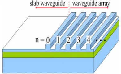
To analyze the problem of nonlinear surface waves, consider a semi-infinite Kerr-nonlinear lattice shown schematically in Figure 1. The discrete nonlinear schrodinger equation (DNLSE) that describes the evolution of complex modal field amplitudes for this system can be written as

2 0

1 0 0 0

d i C

dz

 _ _ __{  } _ ₍₁₎

2

1 1

( ) 0

n

n n n n d

i C

dz

 _ _ _{  }

 

    (2)

(2)

scaled amplitudes



_n as follows

0 0 0 2 2 ˆ n n C E

n n

  



 (3)

where C is the inter-site coupling coefficient in physical units (in Eqs. (1) and (2)), λ0 is the free-space wavelength, η0 is the

free-space impedance, nˆ₂is the nonlinear Kerr coefficient,

and n0 is the linear refractive index of the waveguides

[image:2.595.63.259.265.385.2]

material.

Figure 1: The schematic of a semi-infinite waveguide array.

Of course, equations (1) and (2) are valid only for the first band in the coupled mode approximation which is adequate for this purpose. The ridges formed in the upper cladding lead to an effective refractive index to the right of the boundary larger than that to the left. Hence, the fields associated with the channel waveguides exhibit a higher effective refractive index than that experienced by any propagating modes in the 1D slab waveguides, i.e. the propagation wave vectors for the array region are larger than those of the slab waveguide. As a result, at the boundary, there is no coupling between the slab waveguide modes and the array modes, and the boundary channel field decays exponentially with distance into the slab region with the decay constant approximately that for a single isolated channel. However, this boundary channel does couple via its evanescent field to its nearest neighbor channel.

3. ANALYTICAL SETUP AND RESULTS

T Discrete nonlinear surface waves in a semi-infinite lattice can be numerically found using relaxation and perturbation methods. Let the stationary solution to the Equation (2) of the following form

exp(

)

n

u

n

i Ct







(4) whereis the corresponding propagation constant, and all amplitudes un are assumed to be positive, which corresponds

to an in-phase solution. In the system under consideration, solitons can be found with values of the propagation

constant falling into the semi-infinite gap,

 

2

, where localized solutions are possible in principle.

The family of soliton solutions, found numerically by means of the relaxation method. Total power P carried by the soliton solution peaked at the boundary channel can be written as follow

2

0

n

P









(5)

above power threshold , the 1D surface solitons are strongly localized, and may be approximated by a simple ansatz

exp( )

n A np i Ct



    (6)

where the amplitude is given by

2 2

1

2 4

A    (7)

and

2ln

p



A

(8)

Equation (2) can be rewrite as follow

2

n n n n n

i



  

C





C





  

(9)

By putting the value of equation (4) in equation (9), we get

3

2 n

2

n n n

0 C



C







 



 



(10)

where



₂



_n





_n_₁





_n_₁



2 

_nis the discrete Laplacian in 1-D.

To examine the stability of



_n, we introduce the linearization ansatz

n

Z

n n









(11)

where





1

, and substitute this in to equation (9), it yield the following linearization equation at O( ) :

2

2 2 3

n n n n n n

i



  C



 C



  



Z



(12)

writing



n nin, and linearizing in



, we find

n n n n N





        

    (13)

(3)

0

M N

M





 

 _ 

 (14)

and

 



2



2 n

2 M

_

C

   

C



  

C

(15)

 



2



2 3 n 2

M_ C    C



   C (16)

By the eigenvalues of N the stability of



_n_{is determined.} Let the eigenvalues of N be denoted by id, which implies that

n



is stable if the Im(d) = 0. Because the equation (14) is linear, we can eliminate one of the ‘eigenvectors’, for instant



_n, from which we obtain following eigenvalue problem

2

( )

d

_n _n

M C M C

_ _





 



(17)

4. STABILITY OF SURFACE SOLITON AS A FUNCTION

OF POWER

Using equations (5, 6, 7 & 8), we plot a curve between power P verses propagation constant  for different values of C. P  curve exhibits a minimum which,

in turn, implies that discrete nonlinear surface waves can exist only above a certain power threshold. Below the power threshold no surface waves can be supported.

Below power threshold the eigenvalues of equation (17) bifurcates from the edge of continuous spectrum and give rise to an additional unstable eigenvalue pair, with

Im(d)



0

. At threshold eigenvalues of equation (17) just collide with continuous spectrum. And above power threshold eigenvalues cross the continuous spectrum such that Im(d) = 0.

Linear stability analysis reveals that the surface wave solutions are only stable to the right of the minimum of

P curve, i.e. in the region wheredP d 0, in agreement with the well-known Vakhitov-Kolokolov criterion for continuous media [31 & 32]. In the stable branch, the localization of soliton solutions increases with soliton power and the evanescent field decay into the continuous low index region.

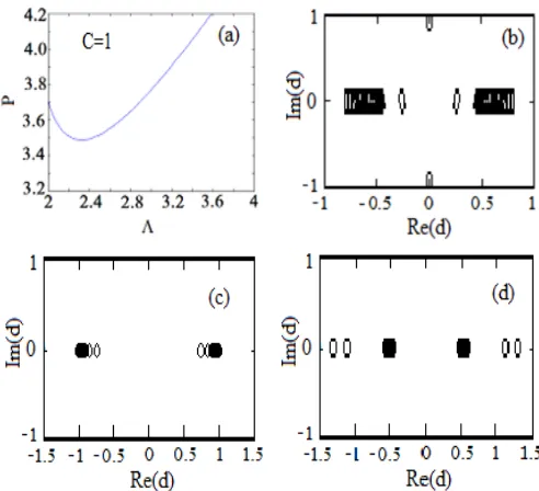
In figure (2(a)), we plot power P as a function of propagation constant



, taking coupling constant C = 1. We clearly found that the minimum in theP  curve occurs at

2.31

  and the threshold power corresponds to this value is 3.495. Figure (2(b), (c) and (d)) verify the value of _also. According to figure (2(b)), when we take  2.11, the

eigenvalues of equation (17) bifurcates from the edge of

continuous spectrum and give rise to an additional unstable eigenvalue pair, with

Im(d)



0

. So no soliton solution found. For  2.31 eigenvalues of equation (17) just

collide with continuous spectrum. For  2.40 eigenvalues

cross the continuous spectrum such that Im(d) = 0, then we found the strong localized solution in form of surface soliton.

Figure 2: (a) Total power (P

constant for an in-phase surface soliton solution peaked at n=0 and C=1. (b),(c) and (d) The structure of eigenvalue at

respectively.

5. DEPENDENCY OF TOTAL POER

P

ON

PROPAGATION CONSTANT



FOR VARIOUS VALUES

OF COUPLING CONSTANATS

[image:3.595.312.558.177.401.2]

(4)

constant curves for various values of coupling constant

6. DEPENDENCY OF THRESHOLD POER

P

ON

COUPLING CONSTANAT

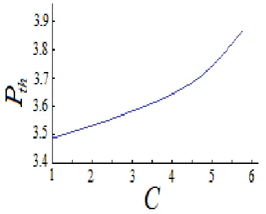
Threshold power (Pth) versus coupling constant (C)

curve shows that if we increase the value of C then the value of Pth is also increased. Which is shown in figure (4). In this

[image:4.595.308.562.186.687.2]

case propagation constant  is taken 2.31

Figure 4: Threshold power (Pth) versus coupling constant

(C) curve.

6. EFFECT OF COUPLING CONSTAT ON THE

INTENSITY AND SHAPE OF SOLITON

We solve equation (10) using Newton-Raphson method for 100 iterations using software MATLAB. We investigate the effect of coupling constant on the intensity and shape of surface Soliton.

Let us set the constants  = 2.5,= 1, n = 6 waveguides and a light beam of intensity 1 is injected in to the zeroth waveguide.

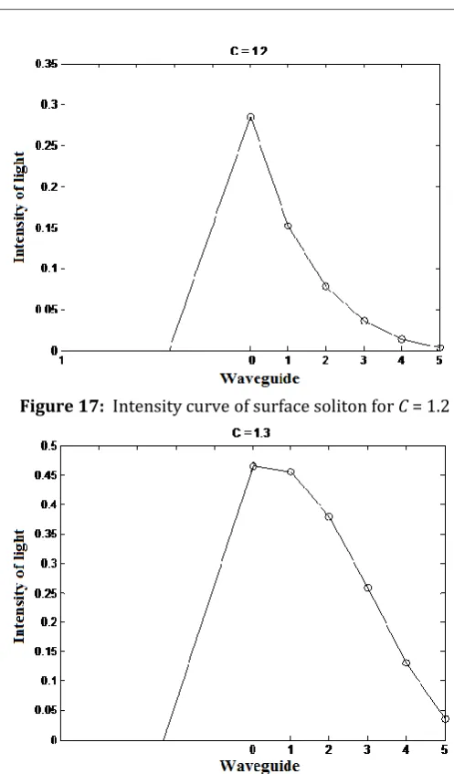
Figures (5) to (18) are plot of intensity of light through 6 waveguides. The intensity of waveguide is given by 2

n

 , where __n is the wave function. It is clear from these figures that if the value of C is increased then the intensity of surface soliton is also increased, but shape of soliton became smoother.

Figure 5: Intensity curve of surface soliton for C = 0

Figure 6: Intensity curve of surface soliton for C = 0.1

[image:4.595.64.258.408.564.2]

(5)

[image:5.595.121.541.58.533.2]

[image:5.595.311.552.96.501.2]

[image:5.595.38.280.104.315.2]

[image:5.595.40.268.334.522.2] [image:5.595.313.547.532.732.2] [image:5.595.41.275.554.755.2]

(6)

[image:6.595.77.548.50.546.2] [image:6.595.305.554.78.502.2]

Figure 15: Intensity curve of surface soliton for C = 1

6. CONCLUSIONS

In this investigation, I have studied the existence of surface Soliton at the interface between a semidiscrete one-dimensional Kerr-nonlinear system and a continuous medium (slab waveguide). I found that discrete nonlinear surface waves can exist only above a certain power threshold. Below the power threshold no surface waves can be supported.

The curve between power P verses propagation constant



for different values of C exhibits a minimum which is called power threshold. Below power threshold the eigenvalues bifurcate from the edge of continuous spectrum and give rise to an additional unstable eigenvalue pair that means no surface waves can exist. At threshold eigenvalues just collide with continuous spectrum. And above power threshold eigenvalues cross the continuous spectrum, that means surface soliton can exist on the interface.

[image:6.595.41.271.110.369.2] [image:6.595.35.279.377.725.2]

(7)

P curve, i.e. in the region wheredP d 0. In the stable branch, the localization of soliton solutions increases with soliton power and the evanescent field decay into the continuous low index region.

I also found that the value of threshold power P is increased, if the value of coupling constant C is increased. In threshold power (Pth) versus coupling constant (C) curve, I found that if

the value of C is increase then the then the value of Pth is also

increased.

More interestingly, I observed that increasing the strength of the coupling C between the waveguides increases the light intensity in the excited waveguide resulting in a smoother soliton .

REFERENCES

[1] A. D. Boardman, M. Bertolotti, and T. Twardowski,

Nonlinear Waves in Solid State Physics (Plenum Press: New York, 1989).

[2] S. Kawata, Near-Field Optics and Surface Plasmon

Polaritons (Springer: Berlin, 2001).

[3] Y. M. Aliev, H. Schluter, and A. Shivarova,

Guided-wave-produced Plasmas (Springer: Berlin, 2000).

[4] S. V. Biryukov, Y. V. Gulyaev, V. V. Krylov, and V. P.

Plessky, Surface acoustic waves in inhomogeneous media (Springer: Berlin, 1995).

[5] K. G. Makris et al., Opt. Lett. 30, 2466 (2005).

[6] Y. V. Kartashov, V. A. Vysloukh, and L. Torner, Phys. Rev.

Lett. 96, 073901 (2006).

[7] M. I. Molina, R. A. Vicencio, and Y. S. Kivshar, Opt. Lett.

31, 1693 (2006).

[8] C. R. Rosberg et al., Phys. Rev. Lett. 97, 083901 (2006).

[9] E. Smirnov et al., Opt. Lett. 31, 2338 (2006).

[10] G. A. Siviloglou et al., Opt. Express 14, 5508 (2006).

[11] Y. V. Kartashov, L. Torner, and V. A. Vysloukh, Opt. Lett.

31, 2595 (2006).

[12] M. I. Molina et al., Opt. Lett. 31, 2332 (2006).

[13] K. Itoh et al., MRS Bulletin 31, 620 (2006).

[14] S. Nolte et al., Appl. Phys. A 77, 109 (2003).

[15] T. Pertsch et al., Opt. Lett. 29, 468 (2004).

[16] A. Szameit et al., Appl. Phys. B 82, 507 (2006).

[17] A. Szameit et al., Opt. Express 15, 1579 (2007).

[18] A. Szameit et al., Appl. Phys. B 87, 17 (2007).

[19] D. Bloemer et al., Opt. Express 14, 2151 (2006).

[22] K. G. Makris, J. Hudock, D. N. Christodoulides, and G. I.

Stegeman, Opt. Lett. 31, 2774 (2006).

[23] Y. V. Kartashov, V. A. Vysloukh, D. Mihalache, and L.

Torner, Opt. Lett. 31, 2329 (2006)

.

[24] Y. V. Kartashov, and L. Torner, Opt. Lett. 31, 2172

(2006).

[25] X. Wang, A. Bezryadina, Z. Chen, and G. I. Stegeman,

Phys. Rev. Lett. 98, 123903 (2007).

[26] A. Szameit,Y. V. Kartashov, F. Dreisow, and T. Pertsch,

Phys. Rev. Lett. 98, 173903 (2007).

[27] Y. V. Kartashov, F. Ye, and L. Torner, Opt. Express 14,

4808 (2006).

[28] I. L. Garanovich, A. A. Sukhorukov, Y. S. Kivshar, and M.

Molina, Opt. Express 14, 4780 (2006).

[29] Y. V. Kartashov, V. A. Vysloukh, A. A. Egorov, and L.

Torner, Opt. Express 14, 4049 (2006).

[30] Y. V. Kartashov, V. A. Vysloukh, A. A. Egorov, and L.

Torner, Opt. Express 14, 12365 (2006).

[31] N. G. Vakhitov, A. A. Kolokolov, Stationary solutions of

the wave equation in a medium with nonlinearity saturation, Izv. Vuz. Radiofiz. 16, 1020 (1973), Translation: Radiophys. and Quant. Electronics 16, 783 (1975).

[32] L. Berge, Wave collapse in physics: principles and

Study of Surface Soliton at the Interface Between a Semidiscrete One Dimensional Kerr Nonlinear System and a Continuous Medium (Slab Waveguide)