From Phillips curve to wage curve
Graafland, J.J.
Tilburg University, CentER
1991
Online at
https://mpra.ub.uni-muenchen.de/21077/
october 1991
From Phillips Curve to Wage Curve
by J.J. Graafland*
Abstract:
In most traditional macro-economic models of the Netherlands the wage equation is specified by a Phillips curve, in which wage growth is negatively related to the unemployment rate. This paper shows, however, that wage formation can better be described by the so-called wage curve, in which the wage level instead of wage growth depends negatively on the unemployment rate.
14 Van Stolkweg, 2585 JR, The Hague The Netherlands
Telephone (070) 3514151 Telefax (070) 3505847
*
The author thanks S.K. Kuipers, and D.A.G. Draper and other colleagues of the Central Planning Bureau for their useful comments.
In policy analysis with traditional macro-economic models of the Netherlands, like the Freia-Kompas model of the Central Planning Bureau (Van den Berg et al., 1988), the wage equation plays an important role. In a standard wage equation private wage growth is explained by the percentage change of consumer prices, labour productivity, the forward shifting of income taxes and social premiums and the change and the level of the difference between the unemployment rate and the frictional unemployment rate. The latter effect is the so-called Phillips curve effect. Simulation results of all kind of government policies depend crucially on these various elements of the wage equation. For example, a reduction of indirect taxes will reduce wages because of its linkage to the consumer price. Similarly, wages will also be reduced when income taxes or social premiums fall.
However, because of the inclusion of the Phillips curve effect these kind of effects are likely to be only relevant in the short and medium term. Since the fall in wages induces a reduction of unemployment, the Phillips curve effect will generate a positive impulse on wage growth, which will continue as long as unemployment lies below its steady state value. Therefore, in the long term the real wage rate will return to its steady state value and so will unemployment. This implies that a permanent change in the tax burden has no long run effects on unemployment.
Recently the Phillips curve has been criticized for several reasons (Blanchflower and Oswald, 1989; Christofides and Oswald, 1989). It is argued that wage formation can better be described by the so-called wage curve, in which wage growth depends only on the change in unemployment and not on the level of unemployment. Unemployment would therefore have a downward influence on wage levels and not on wage growth. This has important policy implications, since it implies that a permanent reduction in tax rates will have long term effects on unemployment, that do not diminish by the Phillips curve effect. The other side of the coin is that unemployment will not automaticly return to the level of frictional unemployment in the long run if other determinants of the wage equation, like the direct or indirect tax rate, remain unchanged.
2. Theoretical background of the Phillips curve and wage curve
The Phillips curve
Much of the literature on empirical research of wage formation stems from the work of Phillips (1958). Phillips started from the proposition that the price of any product changes in response to excess demand. Applying this proposition to the labour market leads to the famous Phillips curve, which relates wage growth to the level of unemployment. Phillips' model is one in which employers bid up wages competitively in order to attract labour away from other firms. When demand for labour is high and there are few unemployed, employers will bid up wage rates rapidly to attract the most productive labour. On the other hand, when labour demand is low and unemployment is high, workers will be reluctant to accept wage cuts and hence wage rates fall only slowly. Phillips therefore notes that the relation between unemployment and the wage growth is likely to be highly non-linear. In addition, Phillips argues that wage growth might also depend on the change in the unemployment rate. In a period of rising business activity, employers will be bidding more vigorously than they would be when the average unemployment rate was the same but business activity was falling. This creates loops in the Phillips curve. This is often labelled the weak Phillips curve effect.
In a subsequent paper Lipsey (1960) builds on the work of Phillips. In contrast to Phillips he argues that the origin of the loops in the macro Phillips curve could be found in the aggregation of micro labour markets, which are affected differently by fluctuations in aggregate demand. A second innovation of Lipsey in the Phillips curve concerned his inclusion of the cost of living index as an explanatory variable.
Phelps (1968) and Friedman (1968) stressed the role of expectations. Whereas Phelps focused on the influence of expectations with respect to wages of other firms, Friedman builds on the paper of Lipsey (1960) and considers the endogeneity of expectations of consumer prices. From his paper the Phillips curve was redefined into the so-called 'expectations augmented' Phillips curve:
(1) _ log w = _ log pce + f (ur, _ ur) fur<0 ; f_ur<0
where w denotes the wage rate, pce is the expected consumption price, and ur the unemployment rate.
over wage growth. The wage outcome is assumed to be a weighted average of wage growth claims of unions and wage growth offers of employers' organisations. The Phillips curve effect is introduced by the assumption that the bargaining power of the union, which determines the weight of unions claims in the wage outcome, is negatively related to the level (and the change) of the unemployment rate. Wage growth claims are assumed to be related to relative changes in consumer prices, labour productivity and employee tax rates, whereas wage growth offers are linked to marginal labour productivity growth, which is determined by relative changes in value added prices, labour productivity and employer tax rates. From these assumptions the following wage growth equation results:
(2) _ log w = a1 _ log py + (1-a1) _ log pc + _ log h + a2 _ log (1-tpw) +
a3 _ log (1-tpl) - a4 ur - a5 _ ur + a6
where py denotes value added price, h labour productivity, tpw the rate of social premiums paid by employers, and tpl the rate of social premiums and income taxes paid by employees.
Equation (2) is still used for policy evaluation in the Netherlands. In the model of the Central Planning Bureau (1989) a1 equals 0., a2 -0.85, a3 -0.25, a4 0.25 and a5 0.45. The only
difference is that in the Freia-Kompas model the weak Phillips curve effect is replaced by a positive influence of the relative change in employment in order to link up with the 'insider-outsider' theory (Carruth and Oswald, 1987; Lindbeck and Snower, 1986). In the model of the University of Groningen (Kuipers et al., 1988) a1 equals 0, a2 -0.86, a3 -0.43, a5 0, whereas the coefficient of the
Phillips curve effect, which is specified as the reciprocal of the unemployment rate, equals 6.64.
The wage curve
In the international literature another route has been followed, which builds on a largely neglected paper of Sargan (1964). In this newer tradition (Oswald, 1982; Nickell and Andrews, 1983; Layard and Nickell, 1986; Dimsdale et al.,1989) the wage equation is derived from microeconomic theory of wage bargaining.1 The main elements of this approach can be summarized as follows.2
Suppose that the wage level is the outcome of a bargaining process between a representative worker and employer and can be represented by the generalized Nash bargaining solution:
1In this paper we only discuss the wage bargaining model. Johnson and Layard (1986) present two additional models
from which wage level curves can be derived. The first model is based on equilibrium between labour supply and labour
demand. Empirical research in Graafland (1991a) shows that this model is rejected for the Netherlands. The second model
is the efficiency wage model. The empirical relevance of this model for the Netherlands is still largely unexplored.
(3) max g = log (u(w)-) + (1- ) log ( (w)-) u'(w)>0 ; '(w)<0 ; 0< <1 ; w u(w)> ; (w)>
where u and denote the utility functions of the worker and employer over wages. The workers' utility is positively related to the wage level, whereas the employers' utility is negatively related to the wage level. The utility levels and are the threat points of the worker respectively employer and reflect their utility obtained during a breakdown of the bargaining process. is an exogenous given parameter, representing the relative bargaining strength of the worker. From the first-order and second order condition of equation (3) it follows that any exogenous variable, that increases the threat point utility of the worker ( ) or decreases the threat point utility of the employers' organisation () will induce a rise in the wage outcome.3
In most of the literature unemployment enters the model through the assumption that the threat point of the worker () is related to the income received if the worker has to search for another job (Blanchflower et al., 1989; Christofides and Oswald, 1989; Graafland, 1991b; Hoel and Nymoen, 1988; Nickell and Andrews, 1983), defined as:
(4) = pru rp w* + (1-pru) w*
where pru denotes the proportion of time spent unemployed before finding a job in another firm, rp
the replacement ratio, and w* the macro wage. As long as the worker has not found another job, he receives an unemployment benefit which is equal to the replacement ratio times the wage rate. In general, the proportion of time spent unemployed before finding a job will be positively related to the macro unemployment rate. Hence, a rise in the unemployment rate will reduce the threat point of the worker and cause a fall in the wage outcome of the bargain.
In other models, like Pissarides (1990), unemployment enters the model through the assumption that the threat point of the employers' organisation depends positively on the macro unemployment rate. Here the argument is that a rise of unemployment will decrease search costs for employers because the average duration of vacancies will diminish. Hence labour turnover costs will fall and this enhances the threat point of the employer.
Either way, the bargaining model implies that unemployment will have a negative influence on the wage level, not on wage growth.4 This is in contrast with the Phillips curve and implies that there will be a stable relation between the wage level and the unemployment rate. This is called the wage curve (Blanchflower and Oswald, 1989). The location of the wage curve will depend on all other exogenous variables, that enter the wage bargaining model. Likely candidates
3For a derivation, see appendix 1.
4One referee noted that the level of the unemployment rate might still influence wage growth in the context of a
bargaining model, if the bargaining parties consider employment in their utility function, and if changes in employment
for these other explanatory variables are producer prices, labour productivity, consumer prices, average tax rates on labour income, and replacement ratios (Graafland, 1991b). Producer prices and labour productivity increase employers' utility ( ) by increasing profits. This induces a reallocation to labour income by increasing wages. Consumer prices and tax rates have an ambiguous influence on wages, because they reduce both marginal and average worker's utility (u'(w) respectively u). Finally, wages will also be positively influenced by the replacement ratio, because this increases the threat point of the worker () by improving his income during a break-down of the bargaining process.
After linearization the solution of the wage bargaining model can be written as a wage level equation, in which the wage level depends on the level of the rate of unemployment and other explanatory variables. Of course this wage level equation can be rewritten as a wage growth equation, in which only the weak Phillips curve effect is relevant. In the context of equation (2) this means that a4 is zero.
As an example of a macro-economic model of the Netherlands with a wage curve we mention MORKMON II (Fase et al., 1990). The wage equation of MORKMON II is specified as:
(5) log w = 0.77 log w-1 - 0.88 _ log pc + 1.05 (log pc - 0.77 log pc-1) + 0.85 (log h -
0.77 log h-1) + 0.90 (tpw - 0.77 tpw-1) + 0.16 tpl - 0.43 ur-½ - 1.41
The coefficient of the lagged wage rate differs from one. Therefore, in the long run a wage curve is obtained with a stable relationship between the level of real wages and the unemployment rate, that shifts with changes in the rate of direct taxes and social premiums paid by employers and employees, the indirect tax rate, and the terms of trade (through the consumer price).
3. Phillips curve versus wage curve: estimation results
In this section we will investigate whether wage formation in the Netherlands exhibits a Phillips curve effect or not. We proceed as follows. First, we will investigate the empirical relevance of the Phillips curve effect in the context of a wage growth equation like equation (2). Second, we will estimate a wage level equation, and compare the statistics of this equation with that of the wage growth equation. Third, we will report some encompassing test statistics of the wage growth and wage level equation.
Estimation results of wage growth equation
2SLS with import prices and lagged values of consumer and producer prices and labour productivity as instruments for current prices and current labour productivity.
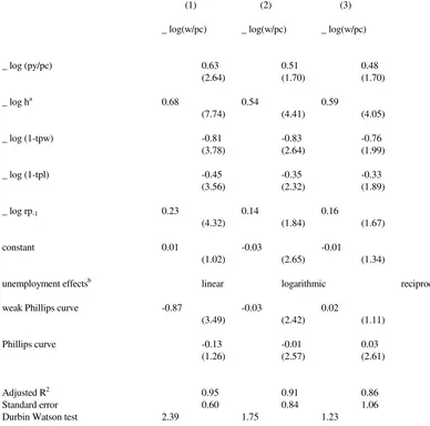
Table 1 presents three estimation results, which differ with respect to the specification of the unemployment effects on wage formation. In column one the unemployment rate is linearly specified, like in the Freia-Kompas model of the Central Planning Bureau (1989). The estimation result shows that only the weak Phillips curve effect has a significant influence on wage growth, whereas the strong Phillips curve effect has not. In the second column the unemployment rate is logarithmicly specified. Now both the weak Phillips curve effect and the strong Phillips curve effect appear to have a significant negative influence on wage growth. However, the overall fit drops. The third column shows the estimation results if a reciprocal specification of the unemployment rate is used, as in Kuipers et al. (1988) and Brunia and Kuper (1990). Again the strong Phillips curve effect is found to be significant, but in comparison with column (1) the overall fit drops. With respect to the other explanatory variables the estimation results are quite
Table 1 Estimation results of wage growth equation
(1) (2) (3)
_ log(w/pc) _ log(w/pc) _ log(w/pc)
_ log (py/pc) 0.63 0.51 0.48
(2.64) (1.70) (1.70)
_ log ha 0.68 0.54 0.59
(7.74) (4.41) (4.05)
_ log (1-tpw) -0.81 -0.83 -0.76
(3.78) (2.64) (1.99)
_ log (1-tpl) -0.45 -0.35 -0.33
(3.56) (2.32) (1.89)
_ log rp-1 0.23 0.14 0.16
(4.32) (1.84) (1.67)
constant 0.01 -0.03 -0.01
(1.02) (2.65) (1.34)
unemployment effectsb linear logarithmic reciprocal
weak Phillips curve -0.87 -0.03 0.02
(3.49) (2.42) (1.11)
Phillips curve -0.13 -0.01 0.03
(1.26) (2.57) (2.61)
Adjusted R2 0.95 0.91 0.86
Standard error 0.60 0.84 1.06
Durbin Watson test 2.39 1.75 1.23
a Labour productivity is related for 25 % to current values and for 75 % to one year lagged values.
b
[image:8.595.83.471.348.732.2]similar. As an indicator for inflation both producer prices and consumer prices play a role in wage formation. Secondly, labour productivity growth appears to be only partly shifted forward into higher wages. Thirdly, changes in both the rate of employers payroll taxes and employees income taxes and social premiums have a positive influence on wage growth, the first effect being about twice as strong as the latter effect. Fourthly, the replacement ratio has a positive influence on wages, which is only significant in the case of a linear specification of the unemployment rate. Finally, it is noted that in all cases the overall fit reduces if other lag structures are used for the unemployment rate or other explanatory variables.5
Estimation results of wage level equation
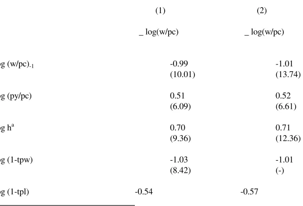
Table 2 reports the estimation results of the wage level equation with a linear unemployment effect.6 For comparison with Table 1 we use the same dependent variable as in the wage growth equation and include the lagged real wage rate as explanatory variable. Note that if the coefficient of the lagged dependent variable differs from minus one, the estimation result implies a partial adjustment process. If the coefficient of the lagged dependent variable does not differ from minus one, the wage growth equation implies a wage level equation without partial adjustment.
Table 2 Estimation results of wage level equation
(1) (2)
_ log(w/pc) _ log(w/pc)
log (w/pc)-1 -0.99 -1.01
(10.01) (13.74)
log (py/pc) 0.51 0.52
(6.09) (6.61)
log ha 0.70 0.71
(9.36) (12.36)
log (1-tpw) -1.03 -1.01
(8.42) (-)
log (1-tpl) -0.54 -0.57
5For estimation results with alternative lag structures, see appendix 3.
6We also estimated wage level equations with a logarithmic and reciprocal unemployment effect, but these equations
appeared to have similar standard errors as the wage growth equations with a logarithmic respectively reciprocal
[image:9.595.91.401.465.676.2](4.75) (8.12)
log rp-1 0.31 0.31
(5.85) (7.92)
ur-1 -1.17 -1.19
(7.13) (9.38)
constant -0.79 -0.81
(4.15) (5.06)
Adjusted R2 0.97 0.97
Standard error 0.46 0.44
Durbin Watson test 2.09 2.09
a
Labour productivity is related for 25 % to current values and for 75 % to one year lagged values.
We present two estimation results. In the first column the coefficient of the rate of social premiums paid by employers exceeds its theoretical maximum value, which equals one (although not significantly). In the second column we therefore restricted the long term coefficient of the rate of social premiums paid by employers to one. From a comparison of the estimation results of Table 2 with those of column (1) in Table 1 it can be seen that estimation of a wage level equation instead of a wage growth equation reduces the standard error. This implies that the wage level specification fits better with Dutch data on wage formation than the wage growth specification.
Encompassing tests
The estimation results in Tables 1 and 2 show that the empirical relevance of the Phillips curve effect is disputable. First, the Phillips curve effect is found to be only significant in the wage growth equations with a logarithmic or reciprocal specification of the unemployment rate. The standard errors of these equations are, however, relatively high compared to that of the wage growth equation in which a linear specification of the unemployment rate is used, and in which the Phillips curve effect is not found to be significant. Second, if we re-estimate the wage equation in the form of a wage level equation with no Phillips curve effect at all, the standard error of the regression is even lower.
These conclusions can be checked by encompassing tests. As a simple preliminary test we use an encompassing test of Davidson and MacKinnon (1981). This test consists of estimating an encompassing wage equation with the fitted values of both alternative equations as regressors:
(6) y = _1 + (1- ) _2
unemployment effects, and the wage level equation. The test statistics are reported in Table 3. In all cases denotes the coefficient of the fitted values of the wage growth equation with a linear specification of unemployment effects.
From the estimation results of in column (1) and (2) in Table 3 it can be seen that the wage growth equation with either a logarithmic or reciprocal specification of the unemployment effects is rejected against the wage growth equation with a linear
Table 3 A simple encompassing test
wage growth equations wage growth versus
wage level equation
linear versus linear versus
logarithmic reciprocal
0.85 0.87 0.27
t-value (4.74) (7.03) (1.72)
specification of the unemployment effects, because differs significantly from zero in these cases (and not from one). On the other hand, from the third column it can be seen that the wage growth equation is rejected against the wage level equation, since differs significantly from one in this case (and not from zero).
A more general test is provided if we estimate encompassing wage equations, in which all coefficients of the underlying equations are freely estimated. In this case the F-test can be used to see which one of the underlying equations can be rejected (Mizon and Richard, 1986). The encompassing equation of the wage growth equations of Table 1 is specified as:
5
(7) _log(w/pc) = bi _log xi + b6 _ur-1 + b7 ur-1 + b8 _log ur-1 + b9 log ur-1 +
i=1
b10 _(1/ur-1) + b11 (1/ur-1) + b12
x1 - x5 denote respectively the ratio between producer prices and consumer prices, labour
productivity, the complements of the employers' social premium rate and the employees' tax and social premium rate, and the replacement ratio. The encompassing wage equation of the wage growth equation with a linear specification of the unemployment effects (column (1) of Table 1) and the wage level equation (column (2) of Table 2) can be specified as:
5 5
(8) _log(w/pc) = ci _log xi + c6 _ur-1 + di log xi + d6 ur-1 + d3 log(w/pc)-1 + d7
The wage growth equation results if the parameters d1 - d5 are zero, whereas the wage level
equation results if c1 - c6 are zero and if d3 differs from zero. The F-test statistics are reported in
Table 4.
Table 4 F-test statisticsa
wage growth equations versus linear logarithmic reciprocal
encompassing wage growth equation (7)
F-test statisticb 1.03 4.29 8.13
wage growth and wage level equation wage growth wage level
versus encompassing wage equation (8)
F-test statisticc 5.14 2.18
a
The F-test statistic is defined as ((SSRi-SSR)/m)/(SSR/(d-1)), where SSRi denotes the sum of squared residuals of the
restricted wage equation, SSR the sum of squared residuals of the encompassing wage equation, m the number of
restrictions, and d the degree of freedoms of the encompassing equation.
b
The critical value of F(m,d) with m=4 and d=11 equals 3.36 at the 5 % level.
c
The critical value of F(m,d) with m=5 (respectively m=6) and d=10 equals 3.33 (3.22) at the 5 % level.
Table 4 yields similar conclusions as Table 3. From the upper part of Table 4 it can be seen that the wage growth equations with a logarithmic and reciprocal specification of the unemployment effects are rejected against the encompassing wage growth equation (7), whereas the wage growth equation with a linear specification of the unemployment effects is not. From the second part of Table 4 it can be seen that the latter is again rejected against the encompassing wage equation (8). On the other hand, the wage level equation is not rejected against the encompassing equation (8). From this we conclude that the standard wage growth equation with a Phillips curve effect gives a deficient description of wage formation in the Netherlands, whereas the wage level equation with a wage curve does not.
This paper shows that the empirical relevance of the Phillips curve effect in the wage equation cannot be confirmed by empirical research. In wage growth equations with a linear specification of the unemployment rate only the change in the unemployment rate has a significant negative effect on wage growth, whereas the level of the unemployment rate is insignificant. If a logarithmic or reciprocal specification is used, the Phillips curve effect is found to have a significant influence on wage growth, but the overall fit worsens. On the other hand, re-estimation of the wage equation in the form of a wage level equation improves the fit. Encompassing tests of the wage level equation and the wage growth equation shows that the wage growth equations with a Phillips curve effect are rejected against a wage level equation with a linear specification of the unemployment rate.
Appendix 1 Derivation of wage bargaining model
The first-order condition for maximum utility is:
(1.1) u'(w)/(u(w)-) + (1- ) '(w)/( (w)-) = 0
Differentiation gives:
(1.2) { u''(w)/(u(w)-) - (u'(w)/(u(w)-))2 + (1- ) ''(w)/( (w)-) -
(1- ) ( '(w)/( (w)-))2} dw = - u'(w)/((u(w)-))2 d - (1- ) '(w)/(( (w)-))2} d
From the second order condition for maximum utility:
(1.3) u''(w)/(u(w)-) - (u'(w)/(u(w)-))2 + (1- ) ''(w)/( (w)-) -
(1- ) ( '(w)/( (w)-))2 < 0
it follows that the term in the left side of equation (1.2) is negative. Since u'(w), u(w)-, and (w)- are positive, whereas
'(w) is negative, it can be concluded that has a positive influence and a negative influence on the wage outcome.
Appendix 2 Data and sources
Most data are from internal sources of the Central Planning Bureau. The replacement ratio is from an internal paper by F. Krapels of the Ministry of Economic Affairs. The time series are constructed as follows:
w = (wb-wk) / (lb - lk -lz) h = (yb-yk) / (lb - lk) tpw = slw / wb tpl = ttl / wb ur = u / ps
where:
wb : wage costs of enterprises
wk : wage costs of the medical sector and other non-private market services
lb : employment of enterprises (labour years)
lk : employment of the medical sector and other non-private market services (labour years)
lz : self-employment (labour years)
yb : value added of enterprises excluding mining and quarrying and real estate (constant prices)
yk : value added of the medical sector and other non-private market services (constant prices)
slw : social premiums, paid by employers
sll : social premiums and direct taxes on wage income, paid by employees in private sector
u : unemployed job-seekers
ps : labour force (persons)
The other series used are defined as:
pc : private consumer price
py : price index of yb-yk
rp : ratio between net government assistance and net average wage rate
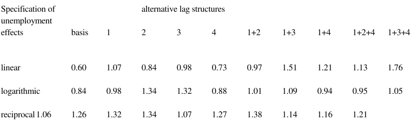
We experimented on four alternative lag structures:
(1)half year lagged producer and consumer prices ; (2)a half year lagged labour productivity ;
(3)a distributed lag in labour productivity with weights .3, .5, and .2 of unlagged, one year lagged, and two year lagged values ;
(4)half year lagged unemployment rates. Because of possible simultaneity between current unemployment and wages, we used the one year lagged specification of the unemployment rate as the instrumental variable for the half year lagged specification.
[image:15.595.84.510.304.438.2]Table 3.1 presents the standard errors of wage equations with these alternative lag structures or combinations of them. The basis column reports the standard errors of the wage growth equations of Table 1.
Table 3.1 Standard errors of wage growth equation with alternative lag structures
Specification of alternative lag structures
unemployment
effects basis 1 2 3 4 1+2 1+3 1+4 1+2+4 1+3+4
linear 0.60 1.07 0.84 0.98 0.73 0.97 1.51 1.21 1.13 1.76
logarithmic 0.84 0.98 1.34 1.32 0.88 1.01 1.09 0.94 0.95 1.05
reciprocal 1.06 1.26 1.32 1.34 1.07 1.27 1.38 1.14 1.16 1.21
References
Berg, P.J.C.M. van den, G.M.M. Gelauff and V.R. Okker (1988), The Freia-Kompas model for the Netherlands: a quarterly macroeconomic model for the short and medium term, Economic Modelling, Vol. 5, no. 3, pp. 170-236
Blanchflower, D.G. and A.J. Oswald (1989), The wage curve, NBER Working Paper no. 3181 Blanchflower, D.G., A.J. Oswald and M.D. Garrett (1989), Insider power in wage determination, NBER Working Paper no. 3179
Brunia, N, and G.H. Kuper (1990), De specificatie van de afwenteling van de collectieve lasten, Maandschrift Economie, 54, pp. 49-55
Carruth, A.A and A.J. Oswald (1987), On union preferences and labor markets models, insiders and outsiders, The Economic Journal, 97, pp. 431-445
Central Planning Bureau (1989), Een verkenning van de Nederlandse economie voor de periode 1991-1994, Werkdocument no. 31
Christofides , L.N. and A.J. Oswald (1989), Real wage determination in collective bargaining agreements, NBER Working Paper no. 3188
Davidson, R. and J.G. MacKinnon (1981), Several tests for model specification in the presence of alternative hypotheses, Econometrica, 49, no. 3, pp. 781-93
Dimsdale, N.H., S.J. Nickell and N. Horsewood (1989), Real wages and unemployment in Britain during the 1930s, The Economic Journal, 99, june, pp. 271-92
Fase, M.M.G., P. Kramer and W.C. Boeschoten (1990), MORKMON II, het DNB kwartaalmodel van de Nederlandse economie, DNB, Monetaire Monegrafieën 11
Friedman, M. (1968), The role of monetary policy, The American Economic Review, Vol. LVIII, no. 1, pp. 1-17
Graafland, J.J. (1988), Hysteresis in unemployment in the Netherlands, De Economist, Vol. 136, pp. 508-523
Graafland, J.J. (1990), Persistent Unemployment, Wages and Hysteresis, dissertation
Graafland, J.J. (1991a), Effecten van marginale belasting- en premiedruk op loonvorming, Maandschrift Economie, forthcoming
Graafland, J.J. (1991b), Insiders and outsiders in wage formation: the Dutch case, Empirical Economics, forthcoming
Hoel, M. and R. Nymoen (1988), Wage formation in Norwegian manufacturing: an empirical application of a theoretical bargaining model, European Economic Review, Vol. 32, pp. 977-997 Johnson, G.E. and P.R.G. Layard (1986), The natural rate of unemployment: explanation and policy, in: O. Ashenfelter and R. Layard (eds.), Handbook of Labor Economics, Vol. II, Elsevier Science Publisher, pp. 921-999
Knoester, A. and N. van der Windt (1987), Real wages and taxation in ten OECD countries, Oxford Bulletin of Economics and Statistics, Vol. 49, no. 1, pp. 151-169
Layard, P.R.G. and S.J. Nickell (1986), Unemployment in Britain, Economica, 53, pp. s121-s169
Lindbeck, A. and D.J. Snower (1986), Wage setting, unemployment and insider-outsider relations, The American Economic Review, Papers and Proceedings, Vol. 76, pp. 235-239
Lipsey, R.G. (1960), The relation between unemployment and the rate of change of money wage rates in the United Kingdom, 1862-1957; a further analysis, Economica, febr., pp. 1-31
Mizon, G.E. and J.F. Richard (1986), The encompassing principle and its application to testing non-tested hypotheses, Econometrica, 54, pp. 657-78
Nickell, S.J. and M. Andrews (1983), Unions, real wages and employment in Britain 1951-79, Oxford Economic Papers, pp. 183-206
Oswald, A.J. (1982), The microeconomic theory of trade unions, The Economic Journal, Vol. 92, pp. 576-595
Phelps, E.S. (1968), Money-wage dynamics and labor-market equilibrium, The Journal of Political Economy, Vol. 76 (4), part II, pp. 678-711
Phillips, A.W. (1958), The relation between unemployment and the rate of change of money wage rates in the United Kingdom, 1861-1957, Economica, Nov., pp. 283-299
Pissarides, C.A. (1990), Equilibrium Unemployment Theory, Basil Blackwell, Oxford