Conservative Interaction of N Internal Waves in Three Dimensions

(1)

http://dx.doi.org/10.4236/ajcm.2014.44029

Conservative Interaction of

N

Internal

Waves in Three Dimensions

Victor A. Miroshnikov

Department of Mathematics, College of Mount Saint Vincent, New York, USA Email: [email protected]

This work is licensed under the Creative Commons Attribution International License (CC BY).

http://creativecommons.org/licenses/by/4.0/

Abstract

The Navier-Stokes system of equations is reduced to a system of the vorticity, continuity, Helm-holtz, and Lamb-Helmholtz equations. The periodic Dirichlet problems are formulated for internal waves vanishing at infinity in the upper and lower domains. Stationary kinematic Fourier (SKF) structures, stationary exponential kinematic Fourier (SKEF) structures, stationary dynamic expo-nential (SDEF) Fourier structures, and SKEF-SDEF structures of three spatial variables and time are constructed in the current paper to treat kinematic and dynamic problems of the three-di- mensional theory of the Newtonian flows with harmonic velocity. Two exact solutions for

con-servative interaction of N internal waves in three dimensions are developed by the method of

de-composition in invariant structures and implemented through experimental and theoretical pro-gramming in Maple™. Main results are summarized in a global existence theorem for the strong solutions. The SKEF, SDEF, and SKEF-SDEF structures of the cumulative flows are visualized by two-parametric surface plots for six fluid-dynamic variables.

Keywords

Existence Theorem, Internal Waves, Invariant Structures, Experimental Programming, Theoretical Programming

1. Introduction

The three-dimensional (3d) Navier-Stokes system of partial differential equations (PDEs) for a Newtonian fluid with a constant density ρ and a constant kinematic viscosity ν in a gravity field g is

(

)

1

, t

p

t ρ ν

∂ _{+ ⋅∇} _{= − ∇ + ∆ +} ∂

v

(2)

0,

∇ ⋅ =v (2)

where ∇=

(

∂ ∂ ∂ ∂x, y,∂ ∂z

)

and _{∆ = ∂ ∂ + ∂ ∂ + ∂ ∂}2 _x2 2 _y2 2 _z2

are the gradient and the Laplacian in the Cartesian coordinate system x=

(

x y z, ,

)

of the 3d space with unit vectors

(

i j k, ,

)

; t is time; v=

(

u v w, ,

)

is a vector field of the flow velocity; g=

(

0, 0,−g_z

)

is a vector field of the gravitational acceleration; pt is a

scalar field of the total pressure.

By a flow vorticity ω=

(

δ κ ω, ,

)

of the velocity field

,

∇ × =v ω (3)

Equation (1) may be written into the Lamb-Pozrikidis form [1] [2]

1

, 2

t

p

t ρ ν

 

∂

+ ∇_ ⋅ + − ⋅ _+ × + ∇× =

∂ _ _ 0

v

v v g x ω v ω (4)

which sets a dynamic balance of inertial, potential, vortical, and viscous forces, respectively. Using a dynamic pressure per unit mass [3]

0 _,

t d

p p p

ρ

−

= − ⋅g x (5)

where p0 is a reference pressure, a kinetic energy per unit mass ke = ⋅v v 2, the 3d Helmholtz decomposition [4] of the velocity field

,

φ

= ∇ + ∇×

v ψ (6)

,

∇ ⋅ =ψ 0 (7)

and the vortex force

, d × = ∇ + ∇×

ω v a (8)

,

∇ ⋅ =a 0 (9)

Equation (4) is reduced to the Lamb-Helmholtz PDE [5]

e b ∇×

∇ + h_e =0 (10) for a scalar Bernoulli potential and a vector Helmholtz potential h_e =

(

fe ge he, ,

)

, respectively,

,

e d e

b p k d

t

φ

∂

= + + +

∂ (11)

, e

t ν ∂

= + +

∂ ψ

h ω a (12)

where φ, d are scalar potentials and ψ=

(

χ η ψ, ,

)

, , ,a=

(

a b c

)

are vector potentials of v and ω v× , re-spectively. The Lamb-Helmholtz PDE (10) sets a dynamic balance between potential and vortical forces of the Navier-Stokes PDE (1), which are separated completely. Reduction of (1) to (10) means the potential-vortical duality of the Navier-Stokes PDE for free flows [3] since writing Equation (10) as

e b

= −∇ =∇× _e

s

n h (13)

shows that a virtual force ns of (1) may be represented both in the potential form ns = −∇be and the vortical

form ns= ∇ ×he. For instance, the potential-vortical duality of (1)-(2) results in formation of the wave-vortex

structures in surface waves [6]-[8].

(3)

zigzag hyperbolic structures were studied to derive the exact solution for interaction of two pulsatory waves of the Korteweg-de Vries equation in [12]. In two dimensions, the stationary kinematic Fourier (SKF) structures with space-dependent structural coefficients, the stationary exponential kinematic Fourier (SKEF) structures, the stationary dynamic exponential Fourier (SDEF) structures, and SKEF-SDEF structures with constant structural coefficients were developed to obtain the exact solutions of the Navier-Stokes system of PDEs for conservative interaction of N internal waves by the experimental and theoretical programming [5].

In the current paper, the SKF, SKEF, SDEF, and SKEF-SDEF structures are extended in three dimensions to examine kinematic and dynamic problems for internal conservative waves in the theory of Newtonian flows with harmonic velocity. The structure of this paper is as follows. The SKF structures are used to compute theo-retical solutions for the velocity components in Section 2. Theotheo-retical solutions for the kinematic potentials of the velocity field and the dynamic potentials of the Navier-Stokes PDE are obtained in Sections 3 and 4, respec-tively, through the SKEF structures. The SDEF structures are constructed in Section 5. In Section 6, the SDEF and SKEF-SDEF structures are used for theoretical computation of the kinetic energy and the dynamic pressure. Decomposition of harmonic variables in a SKEF structural basis is tackled in Section 7. Verification of the ex-perimental and theoretical solutions by the Navier-Stokes system of PDEs and the existence theorem are pro-vided in Section 8. Discussion of significant outcomes and visualization of the developed structures are given in Section 9, which is followed by a summary of main results in Section 10.

2. Velocity Components in the SKF Structures

The following theoretical solutions and admissible boundary conditions of Sections 2-8 were primarily com-puted in Maple™ using experimental programming with lists of equations and expressions for numerical indices and N = 3 in the virtual environment of a global variable Eqe by 33 developed procedures of 1748 code lines.

Theoretical problems for harmonic velocity components u=u x y z t

(

, , ,

)

, v=v x y z t

(

, , ,

)

, w=w x y z t

(

, , ,

)

of cumulative flows v=ui+ +vj wk of a Newtonian fluid are given by vanishing the x-, y-, z-components of the vorticity Equation (3) and the continuity Equation (2), respectively,

0, w v

y z ∂ ₋∂ ₌

∂ ∂ (14)

0, u w z x ∂ ₋∂ ₌

∂ ∂ (15)

0, v u x y ∂ ₋∂ ₌

∂ ∂ (16)

0,

u v w

x y z

∂ ₊∂ ₊∂ ₌

∂ ∂ ∂ (17)

To consider conservative interaction of N internal waves, the cumulative flows are decomposed into superpositions of local flows

(

)

(

)

(

)

1 1 1

, , , , , , , , , , , ,

N N N

n n n

u u x y z t v v x y z t w w x y z t

= = =

=

∑

=

∑

=

∑

(18)

such that the local vorticity and continuity equations are

0,

n n

w v

y z

∂ ₋∂ ₌

∂ ∂ (19)

0,

n n

u w

z x

∂ ₋∂ ₌

∂ ∂ (20)

0,

n n

v u

x y

∂ ₋∂ ₌

∂ ∂ (21)

0,

n n n

u v w

x y z

∂ ₊∂ ₊∂ ₌

(4)

where n=1, 2,,N.

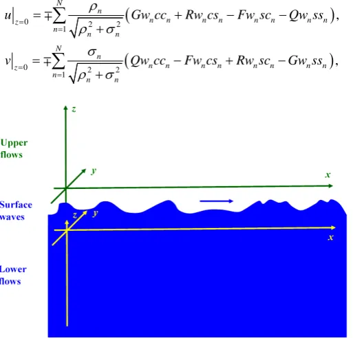
An upper cumulative flow is specified by a Dirichlet condition, which is periodic in the x- and y-directions, through the two-dimensional (2d) SKF structure on a lower boundary z=0 of an upper domainx∈ −∞ ∞

(

,

)

,

(

,

)

, 0,

[

)

y∈ −∞ ∞ z∈ ∞ (seeFigure 1)

(

)

1

0 n n ,

N

n

n n n n n n

z Fw cc w cs Gw sc Rw ss

w ₌ Q

=

+

=

∑

+ + (23)

and a vanishing Dirichlet condition in the z-direction

0.

z

w _=∞ = (24) A lower cumulative flow is identified by a periodic Dirichlet condition on an upper boundary z=0 of a lower domain x∈ −∞ ∞

(

,

)

, ,y∈ −∞ ∞

(

)

, , 0z∈ −∞

(

]

(seeFigure 1)

(

)

1

0 n n ,

N

n

n n n n n n

z Fw cc w cs Gw sc Rw ss

w ₌ Q

=

+

=

∑

+ + (25)

and a vanishing Dirichlet condition in the z-direction

0. z

w _=−∞ = (26) Thus, an effect of surface waves on the internal waves is described by the Dirichlet conditions (23) and (25). While notations of boundary coefficients Fw_n, , , Qw_n Gw_n Rw_n coincide in (23) and (25) for computational simplicity, their values are different for the upper and lower flows, which model internal waves produced by surface waves in atmosphere and ocean. In Equations (23) and (25), a structural notation

( ) ( )

cos cos , cos sin , sin cos , sin sin ,

n n n n n n n n n n n n

cc = α β cs = α β sc = α β ss = α β (27)

is used for kinematic structural functions cc_n, , , cs_n sc_n ss_n, where α_n=ρ_nX_n, β_n=σ_{n n}Y are arguments of the kinematic and dynamic structural functions, X_n= −x Cx t_n −Xa_n, Y_n= −y Cy t Yb_n − _n are propagation va-riables, ρ σ_n, _n are wave numbers, Cx_n, Cy_n are celerities, and Xa_n, Yb_n are initial coordinates for all n.

The experimental solutions show that similar to [5], boundary conditions for u_n, v_n are then redundant since boundary parameters of u_n, v_n depend on boundary parameters of wn for the upper and lower flows,

respec-tively, as

(

)

(

)

0

2 2 1

,

n n N

n

n n n

n n N

n n

n

n n n n z

n n n n n n n n z

n

u R Q

v

Gw cc w cs Fw sc w ss

Qw cc Fw cs Rw sc Gw ss ρ

ρ σ σ ρ σ

=

= =

=

+ − −

−

= + −

=

+

∑



[image:4.595.188.445.446.692.2]

(28)

(5)

Similarly to w, u and v vanish as z→ ±∞

0, 0,

z z

u _=±∞ = v _=±∞ = (29) for the upper and lower cumulative flows, respectively.

Theoretical solutions of (14)-(26) are constructed in the SKF structure p= p x y z t

(

, , ,

)

of three spatial va-riables x, y, z and time t with a general term pn, which in the structural notation may be written as

(

)

( )

1 1

, , , ,

N

n n n n n n n n n

N

n n

fp cc qp c

p p x y z t z z s gp z sc rp z ss

= =

= 

=

∑

_ + + + _ (30)

where first letters f, q, g, r of space-dependent structural coefficients fp_n

( )

z , , , qp_n

( )

z gp_n

( )

z rp_n

( )

z refer to the kinematic structural functions cc_n, , , cs_n sc_n ss_n and a second letter to the expanded variable p. General terms of the velocity components of the local flows in the structural notation become

( )

,

. ,

n n n n n n n n

n n n n n

n

n n n

n

u fu z cc qu z cs gu z sc ru z ss fv z cc qv z cs gv z sc rv z ss

fw z cc qw z cs gw z sc rw z ss v

w

= + + +

(31)

Computation of spatial derivatives of pn gives

( )

,

n n n n n n n

n

n n gp z cc rp z cs fp z sc qp z ss p

x ρ ∂

= _ _

∂ + − − (32)

( )

,

n n n n n n n

n

n n qp z cc fp z cs rp z sc gp z ss p

y σ ∂

= _ _

∂ − + − (33)

d d d d

d d d d .

n n n n

n n n

n

p p p p

cc cs

p f q g r

z z z z sc z ss

∂

= + +

∂ + (34)

Application of (32)-(34) to (31) and substitution in (19)-(22) reduce the four PDEs to three ordinary differen-tial equations (ODEs) and an algebraic equation (AE). For these equations to be satisfied exactly for all inde-pendent variables, indeinde-pendent parameters, structural functions, and structural coefficients of the local flows x, y, z, t, Xa_n, Yb_n, Cx_n, Cy_n, ρ_n, σ_n, cc_n, cs_n, sc_n, ss_n, fu_n, qu_n, gu_n, ru_n, fv_n, qv_n, gv_n,

, n

rv fw_n, qw_n, gw_n, rw_n, all coefficients of the kinematic structural functions must vanish. Vanishing four coefficients of four equations yields 16 equations, which are separated into four systems of four equations each with respect to four groups of the SKF structural coefficients of the velocity components

( )

,

( )

,

( )

n n n

fu z rv z gw z

 

 , qun

( )

z ,gvn

( )

z rw, n

( )

z , gun

( )

z qv, n

( )

z ,fwn

( )

z ,

( )

,

( )

,

( )

n n n

ru z fv z qw z

 

 .

d d d

0, 0, 0, 0,

d d d

n n n

rv fu gw

gw gw fu rv fu rv

z σ z ρ σ ρ ρ σ z

− − = − = + = − + + = (35)

d d d

0, 0, 0, 0,

d d d

n n n

gv qu rw

rw rw qu gv qu gv

− + = − = − + = − − + = (36)

d d d

0, 0, 0, 0,

d d d

n n n

qv gu fw

fw fw gu qv gu qv

− − = + = − = + + = (37)

d d d

0, 0, 0, 0.

d d d

n n n

fv ru qw

qw qw ru fv ru fv

− + = + = − − = − + = (38)

In these four separated systems, first and second equations, which are produced by (19) and (20), are ODEs; third equations, which are generated by (21), are AEs; and fourth equations, which are created by (22), are again ODEs.

Solving the third AEs of separated systems (35)-(38) yields functional relations between structural coeffi-cients:

, , , .

n n n n

n n n n n n n n

n n n n

fu ρ rv qu ρ gv gu ρ qv ru ρ fv

σ σ σ σ

(6)

Substitution of (39) in the second ODEs and addition/subtraction of the first ODEs reduces the second ODEs to identities. Substitution of functional relations (39) into the fourth ODEs reduces them to the following system:

(

)

(

)

(

)

(

)

2 2 2 2

d d

0, 0,

d d

0, 0.

d d

n n

n n v n n n v n

n n

n n v n n n v n

gw rw

rv gv

z z

fw qw

qv fv

z z

ρ σ σ ρ σ σ

+ + = − + + =

(40)

Construct solutions of the first and fourth ODEs in stationary exponential (SE) structures with the following general terms:

(

fv qv gv rv_n, _n, _n, _n,fw qw gw rw_n, _n, _n, _n

)( ) (

z = Fv Qv Gv Rv Fw Qw Gw Rw_n, _n, _n, _n, _n, _n, _n, _n

)

exp

( )

c z_n , (41) where Fv_n, , , , , , , Qv_n Gv_n Rv_n Fw_n Qw_n Gw_n Rw_n, and cn are structural coefficients. Substitution of (41) in

first ODEs of (35)-(38) yields algebraic relations between parameters of the structural coefficients

, , , .

n n n n

n n n n n n n n

n n n n

Fv Qw Qv Fw Gv Rw Rv Gw

c c c c

σ σ σ σ

= = − = = − (42)

Substitution of (41) into (40) returns admissible values of cn for the upper and lower flows, respectively, as

2 2 2 2

, .

n n n n n n n n

c = − = −r ρ +σ c = =r ρ +σ (43) Finally, substitutions of (39) and (41)-(43) into (31) and (18) give the following velocity components of the upper and lower cumulative flows, respectively:

(

)

(

)

(

)

(

)

(

)

(

)

1

, exp

exp

,

. n

n n n n n n n n

n

n n n n n n n n

n

n N

n n

N

n n

n n n

N

n n

n n n n

u Fw Qw

r

v R

Gw cc Rw cs sc ss r z

Qw cc Fw cs sc ss r z

Fw cc Qw cs sc ss r

w Gw

r

w Gw Rw z

ρ σ

=

= + − −

= − + −

= + + +

∑



 



(44)

Thus, the velocity components are resolved through the 3d SKEF structures. If σn =0, then csn=0, 0

n

ss = , and the 3d solution (44) is reduced to the 2d solution in the x z- plane [5]

(

)

(

)

(

)

(

)

1 1

exp , 0, exp ,

N N

n n

n

n n n n n n

n

n n

u Gw ca Fw sa ρ z v w Fw ca Gw sa ρ z

= =

=

=

∑

−  =

∑

+  (45)

where ca_n=cos

( )

α_n , sinsa_n=

( )

α_n . If ρ_n =0, then sc_n=0, 0ss_n= , and the 3d solution (44) is trans-formed into a 2d solution in the y z- plane

(

)

(

)

(

)

(

)

1 1

exp exp ,

0, ,

N

n n n n n

N

n n

n

n n

n

v Qw cb sb z Fw cb

u Fw σ w Qw sb σ z

= =

=

= 

∑

−  =

∑

+  (46)

where cb_n=cos

( )

β_n , sinsb_n=

( )

β_n . Therefore, structural parameters of (44)

( )

2 2 cos , 2 2 sin

n n n n

n _n _n n _n _n

C S

r r

ρ ρ _θ σ σ _θ

ρ σ ρ σ

= = = = = =

+ + (47)

return cosine and sine of local front angles θn with respect to x-axis. In the general case, the local front angles n

θ differ from local celerity angles ϕn, which are defined by

( )

2 2 cos , 2 2 sin .

n n

n n n n

Cx Cy

Cx Cy Cx Cy

ϕ ϕ

= =

+ + (48)

In the case of resonance propagation with ρ σn n =Cx Cyn n, θn =ϕn similar to the case of 2d internal

(7)

3. Kinematic Potentials through the SKEF Structures

Theoretical problems for the kinematic potentials ψ=

(

χ η ψ, ,

)

and φ of v are set by seven global Helm-holtz PDEs (6)-(7)

0, u y z

ψ η

∂ ₋∂ _{− =}

∂ ∂ (49)

0, v z x

χ ψ

∂ ∂

− − =

∂ ∂ (50)

0, w x y

η χ

∂ ∂

− − =

∂ ∂ (51)

0,

x y z

χ η ψ

∂ ₊∂ ₊∂ ₌

∂ ∂ ∂ (52)

0, u x

φ

∂ _{− =}

∂ (53)

0, v y

φ

∂ _{− =}

∂ (54)

0, w z

φ

∂ − =

∂ (55)

since a scalar-vector duality the velocity field admits two descriptions: a scalar description v= ∇φ for ψ=0

and a vector description v= ∇ ×ψ for φ=0. The cumulative kinematic potentials are decomposed into superpositions of local kinematic potentials

(

)

(

)

(

)

(

)

1 1 1 1

, , , , , , , , , , , , , , , .

N N N N

n n n n

x y z t x y z t x y z t x y z t

χ χ η η ψ ψ φ φ

= = = =

=

∑

=

∑

=

∑

=

∑

(56)

The local kinematic potentials are governed by local Helmholtz PDEs

0,

n n

n u

y z

ψ η

∂ ∂

− − =

∂ ∂ (57)

0,

n n

n v

z x

χ ψ

∂ ∂

− − =

∂ ∂ (58)

0,

n n

n w

x y

η χ

∂ ₋∂ ₋ ₌

∂ ∂ (59)

0,

n n n

x y z

χ η ψ

∂ ₊∂ ₊∂ ₌

∂ ∂ ∂ (60)

0, n

n u x

φ

∂ ₋ ₌

∂ (61)

0, n

n v y

φ

∂ ₋ ₌

∂ (62)

0, n

n w z

ϕ

∂ ₋ ₌

∂ (63)

where n=1, 2,,N.

(8)

(

)

1

0 n n n n n n n n ,

z N

n

Fs cc Qscs Gs sc Rs ss

ψ

=

= =

∑

+ + + (64)

where Fs_n, , , Qs_n Gs_n Rs_n are given boundary coefficients. The experimental solutions show that similar to (28)-(29), the vanishing Dirichlet conditions for ψ and the periodic and vanishing Dirichlet conditions for

, ,

χ η φ are redundant.

Construct general terms of the kinematic potentials of the upper and lower flows in the SKF structures by

( )

,

. ,

n n

n n n n n n n n n n n n n n n n

n n n n n n n n n n n

n

n n n n n

fh z cc qh z cs gh z sc rh z ss

fe z cc qe z cs ge z sc re z ss

fs z cc qs z cs gs z sc rs z ss

fp z cc qp z cs gp z sc rp z ss

χ η ψ φ

= + + +

(65)

Computation of derivatives of (65) by (32)-(34) and substitution in (57)-(63) reduce the seven Helmholtz PDEs to four Helmholtz ODEs and three Helmholtz AEs. For these equations to be satisfied exactly for all in-dependent variables, inin-dependent parameters, structural functions, boundary coefficients, and structural coeffi-cients of the upper and lower flows x, y, z, t, Xa_n, Yb_n, Cx_n, Cy_n, ρ_n, σ_n, cc_n, cs_n, sc_n, ss_n, Fw_n,

, n

Qw Gw_n, Rw_n, fh_n, qh_n, gh_n, rh_n, fe_n, qe_n, ge_n, re_n, fs_n, qs_n, gs_n, rs_n, fp_n, qp_n, gp_n, ,

n

rp all coefficients of the kinematic structural functions must vanish. Vanishing four coefficients of seven eq-uations yields 28 eqeq-uations in total for the upper flows and 28 eqeq-uations for the lower flows.

For ψ_n =

(

χ η ψ_n, _n, _n

)

, 16 equations are separated into four systems of four equations each with respect to four groups of the SKF structural coefficients fhn

( )

z re, n

( )

z ,gsn

( )

z , qhn

( )

z ,gen

( )

z rs, n

( )

z ,

( )

,

( )

,

( )

n n n

gh z qe z fs z

 

 , rhn

( )

z ,fen

( )

z qs, n

( )

z , for the upper and lower flows, respectively,

(

)

(

)

(

)

d d

exp 0, exp 0,

d d

d

exp 0, 0,

d

n n n n

n n n n n n n n

n n

re fh

gs Qw r z gs Qw r z

z r z r

gs

fh re Qw r z fh re

z

ρ σ

σ ρ

σ ρ ρ σ

− − = − ± =

+ − = − + + =

  



(66)

(

)

(

)

(

)

d d

exp 0, exp 0,

d d

d

exp 0, 0,

d

n n n n

n n n n n n n n

n n

ge qh

rs Fw r z rs Fw r z

z r z r

rs

qh ge Fw r z qh ge

z

ρ σ

σ ρ

σ ρ ρ σ

− + = − =

− + − = − − + =

   



(67)

(

)

(

)

(

)

d d

exp 0, exp 0,

d d

d

exp 0, 0,

d

n n n n

n n n n n n n n

n n

qe gh

fs Rw r z fs Rw r z

z r z r

fs

gh qe Rw r z gh qe

z

ρ σ

σ ρ

σ ρ ρ σ

− − ± = + ± =

− − = + + =

 



(68)

(

)

(

)

(

)

d d

exp 0, exp 0,

d d

d

exp 0, 0,

d

n n n n

n n n n n n n n

n n

fe rh

qs Gw r z qs Gw r z

z r z r

qs

rh fe Gw r z rh fe

z

ρ σ

σ ρ

σ ρ ρ σ

− + ± = + =

− − − = − + =

  



(69)

where first and second ODEs are produced by (57)-(58), third AEs are generated by (59), and fourth ODEs are created by (60).

For φn, 12 equations are separated into four systems of three equations each with respect to four SKF

struc-tural coefficients _fp_n

( )

z qp, _n

( )

z ,gp_n

( )

z rp, _n

( )

z _ for the upper and lower flows, respectively,

(

)

(

)

d

(

)

exp 0, exp 0, exp 0,

d

n n n

n n n n n n n n n n

n n

fp

fp Fw r z fp Fw r z Fw r z

r r z

ρ σ

− _ _ = − _ _ = − _ = (70)

(

)

(

)

d

(

)

d

n n n

n n n n n n n n n n

n n

qp

qp Qw r z qp Qw r z Qw r z

r r z

ρ σ

(9)

(

)

(

)

d

(

)

d

n n n

n n n n n n n n n n

n n

gp

gp Gw r z gp Gw r z Gw r z

r r z

ρ σ

ρ ± _ = −σ _ _ = − _ = (72)

(

)

(

)

d

(

)

d

n n n

n n n n n n n n n n

n n

rp

rp Rw r z rp Rw r z Rw r z

r r z

ρ σ

ρ ± _ = σ ± _ = − _ = (73)

where first and second AEs are produced by (61)-(62) and third ODEs are generated by (63).

Solving the third AEs of separated systems (66)-(69) yields functional relations between structural coeffi-cients

(

)

(

)

(

)

(

)

exp , exp ,

exp , exp .

n n n n

n n n n n n

n n n n

n n n n n n

n n n n

Qw Fw

fh re r z qh ge r z

Rw Gw

gh qe r z rh fe r z

ρ ρ

σ σ σ σ

ρ ρ

σ σ σ σ

= − + = −

= + = − −

 

(74)

Substitution of (74) in the second ODEs of (66)-(69) and addition/subtraction of the first ODEs reduces the second ODEs to identities. Substitution of (74) into the fourth ODEs reduces them to the following system:

(

)

(

)

(

)

(

)

2 2

d d

exp 0, exp 0,

d d

exp 0, exp 0.

d d

n n

n v n n n n n v n n n n

n n

n v n n n n n v n n n n

gs rs

r re Qw r z r ge Fw r z

z z

fs qs

r qe Rw r z r fe Gw r z

z z

σ ρ σ ρ

+ − = − + + =

+ + = − + − =

 

(75)

Solving the first AEs of separated systems (70)-(73) gives structural coefficients

(

)

(

)

(

)

(

)

exp , exp , exp , exp .

n n n n

n n n n n n n n

n n n n

Fw Qw Gw Rw

fp r z qp r z gp r z rp r z

r r r r

=_ _ =_ _ =_ _ =_ _ (76)

Substitution of (76) in the second AEs and third ODEs of (70)-(73) reduces them to identities.

Construct solutions of the first ODEs of (66)-(69) and (75) in the SE structures with the following general terms for the upper and lower flows, respectively,

(

fe qe ge re_n, _n, _n, _n,fs qs gs rs_n, _n, _n, _n

)( ) (

z = Fe Qe Ge Re Fs Qs Gs Rs_n, _n, _n, _n, _n, _n, _n, _n

)

exp

(

r z_n

)

, (77) where Fe_n, Qe_n, Ge_n, Re_n, Fs_n, Qs_n, Gs_n, Rs_n are structural coefficients. Substitution of (77) in the first ODEs of (66)-(69) yields algebraic relations between parameters of the structural coefficients

2 2

, ,

, .

n n n n

n n n n n n

n n n n

n n n n n n

n n n n

Fe Qs Gw Qe Fs Rw

r r r r

Ge Rs Fw Re Gs Qw

r r r r

σ ρ σ ρ

= − = ± −

= + = ± +



(78)

Substitution of (77) and (78) into (75) reduces them to identities.

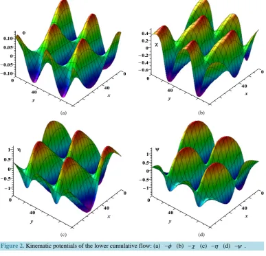
Finally, substitutions of (74), (76)-(78) into (65) and (56) give the following kinematic potentials in the SKEF structures for the upper and lower cumulative flows, respectively,

(

)

(

)

(

)

(

)

(

)

(

)

(

)

(

)

1

exp ,

N

n n

N

n n

N

n

n n n n n n n n

n n n n n n n

n N

n n

n

n n n n n n n n

cc cs sc ss r z

Fs cc Qs cs sc ss r z

cc cs sc ss r z

Fh Qh Gh Rh

Fe Qe Ge Rh

Gs Rs

Fp Qp Gp Rp

χ η ψ φ

=

= + + +

∑



(79)

(10)

2 2

, ,

n n n n

n n n n n n

n n n n

n n n n n n

n n n n

Fh Qh

r r r r

Gh Rh

Gs Qw

r r r r

Rs Fw

Fs Rw Qs Gw

ρ σ ρ σ

= + = −

= ± + = ± −

 

(80)

1 1 1 1

, , , .

n n n n n n n n

n n n n

Fp F Qp Q Gp G Rp R

r w r w r w r w

= = = = (81)

When σ_n =0 and Fs_n=Qs_n=Gs_n=Rs_n=0, (78)-(81) are reduced to the 2d solution in the x-z plane [5]

(

)

(

)

(

)

(

)

1

exp 1

0, ,

1

0, exp .

N

n n n n n

n n

n n n N

n n

Gw c Fw

Gw

a sa z

Fw ca sa z

ρ ψ

χ

ρ

ρ ρ

η φ

=

= = +

= +

− =

∑



 

(82)

When ρ_n =0 and Fs_n=Qs_n=Gs_n=Rs_n=0, (78)-(81) are transformed into a 2d solution in the y-z plane

(

)

(

)

(

)

(

)

1

exp

0, e

1

, 0,

1

xp .

N

n n n n n n

n n n n

N n n

n n

Qw cb Fw

Q

sb z

Fw cb wsa z

ψ

χ σ η

σ

φ σ

σ

=

= − =

+

= =

∑



 

(83)

4. Dynamic Potentials through the SKEF Structures

Definitions of the dynamic vector potential (the Helmholtz potential) h_ψ =

(

fe ge he, ,

)

in the vector description

(

φ =ψ 0

)

are set by three components of temporal derivative (12)

, , .

fe ge he

t t t

χ η ψ

∂ ∂ ∂

= = =

∂ ∂ ∂ (84)

Theoretical problems for the dynamic scalar potential (the Bernoulli potential) b_ψ =be in the vector de-scription are set by three components of the global Lamb-Helmholtz PDEs (10)

0, 0, 0.

be he ge be fe he be ge fe

x y z y z x z x y

∂ ∂ ∂ ∂ ∂ ∂ ∂ ∂ ∂

+ − = + − = + − =

∂ ∂ ∂ ∂ ∂ ∂ ∂ ∂ ∂ (85)

Since the cumulative dynamic potentials are decomposed into superpositions of local dynamic potentials

(

)

(

)

(

)

(

)

1 1

, , , , , , , ,

N N

n n

N N

n n

fe fe x y z t ge ge x y z t

he he x y z t be be x y z t

= =

∑

(86)

the local dynamic potentials are governed by three definitions and three Lamb-Helmholtz PDEs

, , ,

n n n

fe ge he

t t t

χ η ψ

∂ ∂ ∂

= = =

∂ ∂ ∂ (87)

0,

n n n

be he ge

x y z

∂ ∂ ∂

+ − =

∂ ∂ ∂ (88)

0,

n n n

be fe he

y z x

∂ ₊∂ ₋∂ ₌

∂ ∂ ∂ (89)

0,

n n n

be ge fe

z x y

∂ ₊∂ ₋∂ ₌

∂ ∂ ∂ (90)

(11)

re-dundant since boundary parameters of fe ge he be, , , depend on the boundary parameters of w and ψ. Construct a general term of the Bernoulli potential in the SKF structure by

( )

n n n n n

n fB z cc qB z cs gBn z scn n

be = + + +rB z ss (91)

and the SKEF structure l=l x y z t

(

, , ,

)

with a general term ln and structural coefficients Fln, , , Qln Gln Rln

as

(

)

exp

(

)

.

n n n n n n n n n n

l = Fl cc +Ql cs +Gl sc +Rl ss r z (92) Computation of temporal and spatial derivatives of l_n yields

(

)

(

)

(

)

(

)

exp

(

)

,

n

n n n n n n n n n n n n n n n n n n n n n n n n n n n n n

l

Cx Gl Cy Ql cc Cx Rl Cy Fl cs

t

Cx Fl Cy Rl sc Cx Ql Cy Gl ss r z

ρ σ ρ σ

∂ 

= −_ − + − +

∂



+ − + + _ 

(93)

(

)

exp

(

)

,

n

n n n n n n n n n n

l

Gl cc Rl cs Fl sc Ql ss r z x ρ

∂

= + − −

∂  (94)

(

)

exp

(

)

,

n

n n n n n n n n n n

l

Ql cc Fl cs Rl sc Gl ss r z y σ

∂

= − + −

∂  (95)

(

)

exp

(

)

.

n

n n n n n n n n n n

l

r Fl cc Ql cs Gl sc Rl ss r z z

∂

= + + +

∂   (96)

Application of (93) to (87) and (79) gives the following Helmholtz potentials in the SKEF structures for the upper and lower cumulative flows, respectively,

(

)

(

)

(

)

(

)

(

)

(

)

1

exp ,

n n n n n n n n n

n n n

N

n N

n

n n n

N

n n n

n

cc cs sc ss

cc cs sc

fe FF QF GF RF r z

ss

FH cc QH

ge FG QG GG RG r z

he cs GH sc RH ss r z

=

= + + +

∑



(97)

where structural coefficients are

, ,

n n n n n n n n n n n n n n n n n n n n n n n n n n n n

FF Cx Gh Cy Qh QF Cx Rh Cy Fh

GF Cx Fh Cy Rh RF Cx Qh Cy Gh

ρ σ ρ σ

= − − = − +

= − = + (98)

, ,

FG Cx Ge Cy Qe QG Cx Re Cy Fe

GG Cx Fe Cy Re RG Cx Qe Cy Ge

ρ σ ρ σ

= − − = − +

= − = + (99)

, ,

, .

FH Cx Gs Cy Qs QH Cx Rs Cy Fs

GH Cx Fs Cy Rs RH Cx Qs Cy Gs

ρ σ ρ σ

= − − = − +

= − = + (100)

Computation of derivatives of (97) and (91) by (94)-(96) and (32)-(34), respectively, and substitution in (88)- (90) reduce the three Lamb-Helmholtz PDEs to two Lamb-Helmholtz AEs and one Lamb-Helmholtz ODE. For these equations to be satisfied exactly for all independent variables, independent parameters, structural functions, boundary coefficients, and structural coefficients of the upper and lower flows x, y, z, t, Xa_n, Yb_n, Cx_n, Cy_n,

, n

ρ σ_n, cc_n, cs_n, sc_n, ss_n, FF_n, QF_n, GF_n, RF_n, FG_n, QG_n, GG_n, RG_n, FH_n, QH_n, GH_n, ,

n

RH fB_n, qB_n, gB_n, rB_n, all coefficients of the kinematic structural functions must vanish. Vanishing four coefficients of three equations yields 12 equations in total for the upper flows and 12 equations for the low-er flows, which are separated into four systems of three equations each with respect to four SKF structural coef-ficients fBn

( )

z qB, n

( )

z ,gGn

( )

z rB, n

( )

z  for the upper and lower flows, respectively,

(

)

(

)

(

)

(

)

(

)

(

)

exp 0, exp 0,

d

exp 0,

d

n n n n n n n n n n n n n n n

n n n n n

fB r GG RH r z fB r QF RH r z

fB

GG QF r z

z

ρ σ σ ρ

ρ σ

− + ± + = − + − =

+ − =

  

(12)

(

)

(

)

(

)

(

)

(

)

(

)

exp 0, exp 0,

d

exp 0,

d

n n n n n

qB r RG GH r z qB r FF GH r z

qB

RG FF r z

z

ρ σ σ ρ

ρ σ

− + ± − = + − =

+ + =

  

 (102)

(

)

(

)

(

)

(

)

(

)

(

)

exp 0, exp 0,

d

exp 0,

d

n n n n n

gB r FG QH r z gB r RF QH r z

gB

FG RF r z

z

ρ σ σ ρ

ρ σ

+ ± + = − + + =

− + =

  

 (103)

(

)

(

)

(

)

(

)

(

)

(

)

exp 0, exp 0,

d

exp 0,

d

n n n n n

rB r QG FH r z rB r GF FH r z

rB

QG GF r z

z

ρ σ σ ρ

ρ σ

+ ± − = + + =

+ − + =

  

 (104)

where first and second AEs are produced by (88)-(89) and third ODEs are generated by (90).

Solving the first AEs of separated systems (101)-(104) gives the following Bernoulli potentials in the SKEF structures for the upper and lower cumulative flows, respectively,

(

)

(

)

1

exp ,

n n n n n n

N

n

n n n

cc cs sc

be FB QB GB RB ss r z

=

∑

+ + +  (105)

where structural coefficients are

, ,

, .

n n n n

n n n n n n n n n n

n n n n

n n n n n n n n n n

n n n n

FB Cx Gw Cy Qw QB Cx Rw Cy Fw

r r r r

GB Cx Fw Cy Rw RB Cx Qw Cy Gw

r r r r

ρ σ ρ σ

   

= ± − −  = ± − + 

   

   

= ±_ − _ = ±_ + _

   

(106)

Substitution of (106) in the second AEs and third ODEs of (101)-(104) reduces them to identities. The Ber-noulli potential (105)-(106) does not depend on boundary coefficients of the kinematic potentials Fs_n, Qs_n,

, n

Gs Rs_n since ψ of (79) generates the SKEF solution of the homogeneous problem ∇ × =ψ 0.

In the scalar description, ψφ =0, hφ =0 and integration of the Lamb-Helmholtz PDE (10) returns the

Ber-noulli equation [2]

( )

0,

d e

be p k f t

t

φ =∂_∂φ+ + + = (107)

where φ φ= _φ and an arbitrary function of time f t

( )

vanishes for the SKEF structures because of the vanish-ing Dirichlet conditions (24) and (26). Usvanish-ing the scalar-vector duality, the Lamb-Helmholtz PDE (10) reads

.

b be be be be be

t t

t t t

ψ ψ ∂ ∂ ∂ φ ∂φ

∇ + = ∇ + = ∇ + ∇ + ∇ + +

∂ ∂

∂  

∇ × ∇ × ∇ × = = ∇ = ∇ =

∂  ∂ 

∂   0

ψ _ψ v

h (108)

where ψ ψ= ψ. Integration of (108) returns dual formulas for the global and local Bernoulli potentials ,

be t

φ

∂ = −

∂ (109)

n n be

t

φ

∂ = −

∂ (110)

since an integration constant again vanishes for the SKEF structures in agreement with (24) and (26). Therefore, computation of be by (110), (79), and (93) also results in (105)-(106).