Cyber Crime based Curve Fitting Analysis in Internet
Traffic Sharing in Computer Network
Diwakar Shukla
[1], Kapil Verma
[2], Jayant Dubey
[3]and Sharad Gangele
[4] [1]Deptt. of Mathematics and Statistics, Sagar University, Sagar M.P., India.
Associate Member, DST-Centre for Interdisciplinary Mathematical Science, Banaras Hindu University, Varanasi, U.P, India.
[2]
, Deptt. of Computer Science, M. P. Bhoj (Open) University, Bhopal, M.P, India. [3]
Deptt. Of Business Studies, B.T. Institute of Research and Technology, Seronja, Sagar, M.P., India [4]
Deptt. of Statistics, M.B. Khalsa College, Indore, M.P., India
ABSTRACT
Many well-developed countries are having broadband services for there network connection but under developed countries are still having the dial-up-setup connection network. The cyber crime users are growing fast in the entire world and correspondingly the cyber criminals are also growing. The crime is performed by the users cyber only when the connectivity through internet is made. This paper extends the approach of interrelationship between traffic sharing and blocking probability of network between operators subject to conditions the user attracts for cyber crimes. The Markov chain model based approach provides a complicated relationship. This paper adopts a simplified form of same relationship assuming linearity among variables. Least square method is used to generate linear relationship in presence of cyber crime using coefficient of determination and 99 percents confidence interval it has been proved that the approximation is best.
Keywords
Cyber Criminals [CC]
1.
INTRODUCTION
The use if internet and cyber crime are highly co-related factors. The internet service providers may use technique of cyber crime to improve upon their customers proportions. Cyber crime may be a hidden force used to generate internet users. The cyber crimes are like hacking, unwanted mailing, black mailing, threating, cheating to other through networks. Naldi (2002) has used Markov chain model for establishing the relationship between traffic sharing and blocking probability of network. Shukla and Thakur (2007) has extended the approach of Naldi (2002) by introducing the concept of cyber crime. They derived expressions for traffic sharing and
blocking probability in complicated form. This paper uses least square curve fitting theory to express the same in simplified form in cyber crime setup. The values of traffic are generates from the Markov chain model and least square principle is applied on generated data to obtained an approximate linear relationship.
2.
A REVIEW
3.
DEFINING A SYSTEM
NC
C
1-c1 c2
1-L1
1-L2
O1 O2
L1
L2
L p1 A L p2 A
A 1 1
1
Transition probability matrix is
states X (n)
1 2
1
1 1 1
2
2 2 2
1
1 1
2 2
0 1 1 0
1 0 1 0
0 0 1 0
0 0 1 0
0 0 0 0 1
A A
A A
n
O O NC C A
O
L p L L p
O
L p L L p
X NC c c C c c A
3.1 Some Results for n
thAttempts
The starting conditions (state distribution before the call attempt) are ( 0) 1 ( 0) 2 ( 0) ( 0) 1 ...(3.1) 0 0
P X O p
P X O p
P X NC
P X A
Theorem 3.1 : If users attempt are between O1 and O2 then the
nth step transitions probability is
( )1 1 2
1 ( )
1 2 1 2
( )
2 1 2
1 ( )
2 1 1 2 1 1 1 ...(3.2) 1 1 1 n n n A n n n A n n n A n n n A
P X O p L L p even
P X O p L L L p odd
P X O p L L p even
P X O pL L L p odd
4.
QUALITY OF SERVICE [QoS]
There are various categories type of user as (i) Faitful user [FU]-A user who is faithful to an operator O1 otherwise, he goes
to abandon state but does not attempt for O2. The converse of it
may as he attempt for O2 and goes to state A. This describeds
faitful users for operator O1 and O2 (ii) Impatient user [IU]-
User who moves between the two operators O1 and O2 only all
the time until call completes or abandon the process. (iii) Non cyber criminals [NCC] (IV) Cyber Criminals [CC]. Cyber Criminals are two types (a) Non-Serious Cyber Criminals [NSCC] (b) Serious Cyber Criminals [SCC]. The quality of services provides by operators is a function of blocking probabilities (L1 and L2) faced by operators in the network.
More and more blocking probability leads to lesser quality of service for users.
5.
TRAFFIC
SHARING
AND
CALL
CONNECTION
5.1
Traffic Sharing by Non-Cyber Criminals
[NCC]
2 1 1 1 2 2 1 2 1 2 22 1 2
1
1 1
1 1
...(5.1)
1 1 1 1
n A Even A n NCC n A A L c
p L L p
L L p P
p L p L L p
1 1 2
2
1 1 2
2 1 2
1 1 1
...(5.2)
1 1 1
1 1 A n Odd n A NCC A
L c p p L p
P L L p
L L p
Similar for O
2
2
2
1 1
2 2 1 2 2
0 0
1 ...(5.3)
n n
n
N C C i i
i even i even
P L c P X O P X O
2 1 2 1 2 22 1 2
2 2
1 1 2
1
1 1
1 1 1 ...(5.4)
1 1 1
A n Even n A NCC n A A L c
L L p
P p L L p
pL p L L p
2 1 2
2 2
1 2
2 1 2
1
1
1
...(5.5)
1
1
1
1
A n Odd n A NCC AL c
p
pL
p
P
L L
p
L L
p
5.2 Traffic Sharing By Cyber Criminals [CC]
1 1 2 1 2 21 1 2
2 2
2 1 2
1 1
1 1
1 1 ...(5.6)
1 1 1 1
A n Even n A C C n A A L c
L L p
P p L L p
p L p L L p
1 1 2
2
1 1 2
2 1 2
1
1
1
1
...(5.7)
1
1
1
1
A n Odd n A CC AL
c
p
p L
p
P
L L
p
L L
p
Similar for O
2
2 1 2 2 2 2 2 0 0 1 1 ...(5.8) n n n i i C C i ii even i even
L c
P
P X O P X O
2 1 2 1 2 22 1 2
2 2
1 1 2
1 1
1 1
1 1 1 ...(5.9)
1 1 1
A n Even n A CC n A A L c
L L p
P p L L p
pL p L L p
2 1 2
2
2 1 2
2 1 2
1 1 1 1
...(5.10) 1 1 1 1 A n Odd n A CC A
L c p pL p
P L L p
L L p
5.3 Traffic Sharing By Non-Serious Cyber
Criminals [NSCC]
1 1 1 2
3 2 1 1 2 2 1 2
1 1 1 1
...(5.11) 1 1 1 1 A Even n n
N S CC
A
A
L c c P p L p
P
L L p
L L p
Similar for O
2
2 1 1
3 3 2 2 2 0 0
1
1
...(5.12)
n n n i i NSCC i ii even i even
L
c c
P
P X
O
P X
O
2 1 1 1
3 2 1 1 2 2 1 2
1 1 1 1
...(5.13) 1 1 1 1 A Even n n NSCC A A
L c c p pL p
P
L L p
L L p
2 1 1
2 1 2
2
2 1 2
3 2
1 1 2
1 1
1 1
1 1 1 ...(5.14)
1 1 1
A
n Odd
n
A N S CC
n
A A
L c c
L L p
P p L L p
pL p L L p
5.4 Traffic Sharing By Serious Cyber
Criminals [SCC]
1 1 2
3 2 1 1 2 2 2 1 2
1
1
1
...(5.15)
1
1
1
1
1
1
E ven n nS C C
A A
A
L
c
c
P
L L
p
p
p L
p
L L
p
1 1 2
2 1 2
2
1 1 2
3 2
2 1 2
1 1 1
1 1
1 1 ... 5.16
1 1 1 1
A n O dd n A S CC n A A
L c c
L L p
P p L L p
p L p L L p
Similar for O
2
2 1 2
3 3
2
2 2
0 0
1
1
1
...(5.17)
n n n
i i
S C C
i i
i even i odd
L
c
c
P
P X
O
P X
O
2 1 2 1
3 2
2 1 2
2 1 2
1 1 1 1 1
...(5.18) 1 1 1 1 A n Even n A S C C
A
L c c p pL p
P L L p
L L p
2 1 2
2 1 2
2
2 1 2
3 2
1 1 2
1 1 1
1 1
1 1 1 ...(5.19)
1 1 1
A n O dd n A S CC n A A
L c c
L L p
P p L L p
pL p L L p
6. BEHAVIOR OVER LARGE NUMBER
OF ATTEMPTS
1
lim
11 2
n n
P
P
, i
,
1 11 2 2
1 2
1
1 1 ...(6.1)
1 1 A
NCC
A
L c
P p p L p
L L p
2 1
2 2 1
1 2
1
1 1 ...(6.2)
1 1 A
NCC
A L c
P p pL p
L L p
1 11 2 2
1 2
1 1
1 1 ...(6.3)
1 1 A
CC
A
L c
P p p L p
L L p
2 12 2 1
1 2
1 1
1 1 ...(6.4)
1 1 A
CC
A
L c
P p pL p
L L p
1 1 1
1 2 2
1 2
1 1
1 1 ...(6.5)
1 1 A
NSCC
A
L c c
P p p L p
L L p
2 1 1
2 2 1
1 2
1 1
1 1 ...(6.6)
1 1 A
NSCC
A
L c c
P p pL p
L L p
1 1 2
1 2 2
1 2
1 1 1
1 1 ...(6.7)
1 1 A
SCC
A
L c c
P p p L p
L L p
2 1 2
2 2 1
1 2
1 1 1
1 1 ...(6.8)
1 1 A
SCC
A
L c c
P p pL p
L L p
7. LEAST SQUARE CURVE FITTING
We suggest a linear relationship where a, b are constants
1
.
1....(7.1)
P
a b L
Let (
(
P L
1 , 1i i)
i
1, 2,3....
n
be n observations generated from equation (6.1, 6.3, 6.5, 6.7) keeping values fixed for p, pAand L2. Suppose n=9 and blocking probabilities for L1 are (0.1,
0.2, 0.3, 0.4, 0.5, 0.6, 0.7, 0.8, 0.9) then using (8.1), the generated data of
P
1 is in table (1, 2, 3, 4, 5 and 6). TheP
1
is obtained using line equation (8.4) witha b,
.
8. FITTING THE STRAIGHT LINE
We suggest an approximate the relationship between parameter P1 and L1 through a straight line
P
1a
b L
.
1
. The normal equations are1 1
1 1
2
1 1 1 1
1 1
.
...(8.1)
.
n n i i i n n i i i iP
n a
b
L
P L
a
L
b
L
By solving the above equation the least square estimate are a and b are (denoted as
a b
,
): 1 1 1 1
1
...(8.2)
n n i i ia
P
b
L
n
1 1 1 1
1 1 2 2 1 1 1 1
(
)(
)
.... (8.3)
(
)
n n i i i n n i in
P L
P
L
b
n
L
L
Where n is the number of observations in sample (n) and the resultant straight line is
1 1
....(8.4)
P
a b L
The coefficient of determination (COD) is defined as
2 1 1 2 1 1
(
)
COD=
...(8.5)
(
)
i iP
P
P
P
Where
P
11
P
1in
is mean of original data of P1 obtainedthrough Markov chain model. The term
P
1a b L
.
1
is the estimated value give observation L1. The COD lies between 0 to1. If the line is good fit then it is near to 1. We generate pair of value (L1, P1) from express tables (1, 2, 3, 4, 5, 6) by providing
few fixed input parameter
Table 1 (By expression 6.1)
Fixed parameter p=0.4, L2=0.3, pA=02, C1=0.3
L1 0.1 0.2 0.3 0.4 0.5 0.6 0.7 0.8 0.9
P1 0.1498 0.1358 0.1212 0.1061 0.0903 0.0738 0.0566 0.0386 0.0197
1
P
0.1529 0.1366 0.1204 0.1042 0.0888 0.0717 0.0555 0.0393 0.0231 COD=0.9977
1 1 1 1
0.16908;
0.16222;
.
;
0.16908
0.16222.(
)
...(8.4.1)
a
b
P
a
b L
P
L
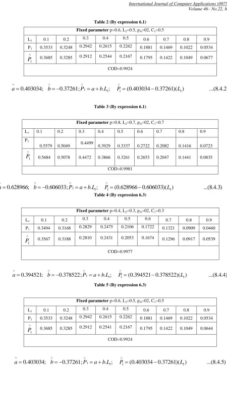
Table 2 (By expression 6.1)
Fixed parameter p=0.6, L2=0.5, pA=02, C1=0.5
L1 0.1 0.2 0.3 0.4 0.5 0.6 0.7 0.8 0.9
P1 0.3533 0.3248 0.2942 0.2615 0.2262 0.1881 0.1469 0.1022 0.0534
1
P
0.3685 0.3285 0.2912 0.2544 0.2167 0.1795 0.1422 0.1049 0.0677 COD=0.99241 1 1 1
0.403034;
0.37261;
. ;
(0.403034 0.37261)( )
...(8.4.2)
a
b
P
a
b L
P
L
Table 3 (By expression 6.1)
Fixed parameter p=0.8, L2=0.7, pA=02, C1=0.7
L1 0.1 0.2 0.3 0.4 0.5 0.6 0.7 0.8 0.9
P1
0.5579 0.5049 0.4499 0.3929 0.3337 0.2722 0.2082 0.1416 0.0723
1
P
0.5684 0.5078 0.4472 0.3866 0.3261 0.2653 0.2047 0.1441 0.0835 COD=0.99811 1 1 1
0.628966;
0.606033;
. ;
(0.628966 0.606033)( )
...(8.4.3)
a
b
P
a b L
P
L
Table 4 (By expression 6.3)
Fixed parameter p=0.4, L2=0.3, pA=02, C1=0.3
L1 0.1 0.2 0.3 0.4 0.5 0.6 0.7 0.8 0.9
P1 0.3494 0.3168 0.2829 0.2475 0.2106 0.1722 0.1321 0.0909 0.0460
1
P
0.3567 0.3188 0.2810 0.2431 0.2053 0.1674 0.1296 0.0917 0.0539 COD=0.99771 1 1 1
0.394521;
0.378522;
. ;
(0.394521 0.378522)( )
...(8.4.4)
a
b
P
a
b L
P
L
Table 5 (By expression 6.3)
Fixed parameter p=0.6, L2=0.5, pA=02, C1=0.5
L1 0.1 0.2 0.3 0.4 0.5 0.6 0.7 0.8 0.9
P1 0.3533 0.3248 0.2942 0.2615 0.2262 0.1881 0.1469 0.1022 0.0534
1
P
0.3685 0.3285 0.2912 0.2541 0.2167 0.1795 0.1422 0.1049 0.0644 COD=0.99241 1 1 1
0.403034;
0.37261;
. ;
(0.403034 0.37261)( )
...(8.4.5)
a
b
P
a
b L
P
L
[image:5.595.59.510.34.842.2] [image:5.595.59.517.86.472.2] [image:5.595.78.513.437.771.2]Table 6 (By expression 6.3)
Fixed parameter p=0.8, L2=0.7, pA=02, C1=0.7
L1 0.1 0.2 0.3 0.4 0.5 0.6 0.7 0.8 0.9
P1 0.2391 0.2164 0.1928 0.1684 0.1433 0.1166 0.0892 0.0607 0.0313
1
P
0.2436 0.2176 0.1916 0.1657 0.1397 0.1137 0.0877 0.0618 0.0358COD=0.9981
1 1 1 1
0.269557;
0.25973;
. ;
(0.269557 0.25973)( )
...(8.4.5)
a
b
P
a
b L
P
L
Table 7 (By expression 6.5)
Fixed parameter p=0.4, L2=0.3, pA=02, C1=0.3
L1 0.1 0.2 0.3 0.4 0.5 0.6 0.7 0.8 0.9
P1 0.1048 0.0955 0.0849 0.0742 0.0632 0.0516 0.0396 0.0277 0.0138
1
P
0.1077 0.0956 0.0843 0.0729 0.0616 0.0502 0.0389 0.0275 0.0162 COD=0.99761 1 1 1
0.118356;
0.11356;
. ;
(0.118356 0.11356)( )
...(8.4.7)
a
b
P
a
b L
P
L
Table 8 (By expression 6.5)
Fixed parameter p=0.6, L2=0.5, pA=02, C1=0.5
L1 0.1 0.2 0.3 0.4 0.5 0.6 0.7 0.8 0.9
P1 0.1767 0.1624 0.1471 0.1307 0.1131 0.0941 0.735 0.0511 0.0267
1
P
0.1829 0.1643 0.1456 0.1277 0.1084 0.0897 0.0711 0.0525 0.0338 COD=0.99251 1 1 1
0.201517;
0.18631;
. ;
(0.201517 0.18631)( )
...(8.4.8)
a
b
P
a
b L
P
L
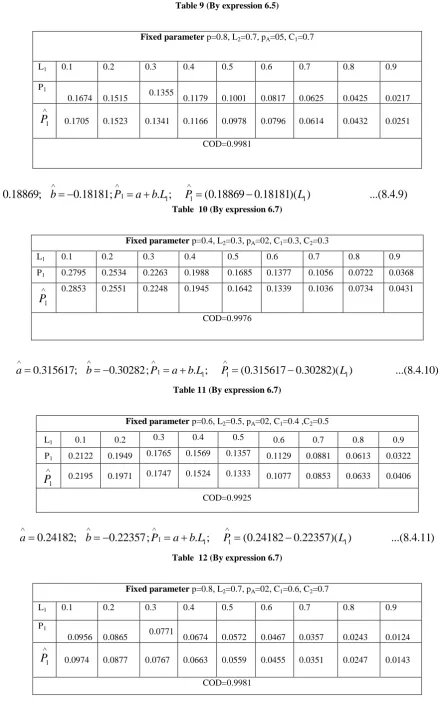
[image:6.595.87.512.96.662.2]Table 9 (By expression 6.5)
Fixed parameter p=0.8, L2=0.7, pA=05, C1=0.7
L1 0.1 0.2 0.3 0.4 0.5 0.6 0.7 0.8 0.9
P1
0.1674 0.1515 0.1355 0.1179 0.1001 0.0817 0.0625 0.0425 0.0217
1
P
0.1705 0.1523 0.1341 0.1166 0.0978 0.0796 0.0614 0.0432 0.0251 COD=0.99811 1 1 1
0.18869;
0.18181;
. ;
(0.18869 0.18181)( )
...(8.4.9)
a
b
P
a b L
P
L
Table 10 (By expression 6.7)
Fixed parameter p=0.4, L2=0.3, pA=02, C1=0.3, C2=0.3
L1 0.1 0.2 0.3 0.4 0.5 0.6 0.7 0.8 0.9
P1 0.2795 0.2534 0.2263 0.1988 0.1685 0.1377 0.1056 0.0722 0.0368
1
P
0.2853 0.2551 0.2248 0.1945 0.1642 0.1339 0.1036 0.0734 0.0431
COD=0.9976
1 1 1 1
0.315617;
0.30282;
. ;
(0.315617 0.30282)( )
...(8.4.10)
a
b
P
a
b L
P
L
Table 11 (By expression 6.7)
Fixed parameter p=0.6, L2=0.5, pA=02, C1=0.4 ,C2=0.5
L1 0.1 0.2 0.3 0.4 0.5 0.6 0.7 0.8 0.9
P1 0.2122 0.1949 0.1765 0.1569 0.1357 0.1129 0.0881 0.0613 0.0322
1
P
0.2195 0.1971 0.1747 0.1524 0.1333 0.1077 0.0853 0.0633 0.0406 COD=0.99251 1 1 1
0.24182;
0.22357;
. ;
(0.24182 0.22357)( )
...(8.4.11)
a
b
P
a
b L
P
L
Table 12 (By expression 6.7)
Fixed parameter p=0.8, L2=0.7, pA=02, C1=0.6, C2=0.7
L1 0.1 0.2 0.3 0.4 0.5 0.6 0.7 0.8 0.9
P1
0.0956 0.0865 0.0771 0.0674 0.0572 0.0467 0.0357 0.0243 0.0124
1
[image:7.595.70.514.72.798.2] [image:7.595.92.508.460.769.2]1 1 1 1
0.107823;
0.10389;
. ;
(0.107823 0.10389)( )
...(8.4.12)
a
b
P
a
b L
P
L
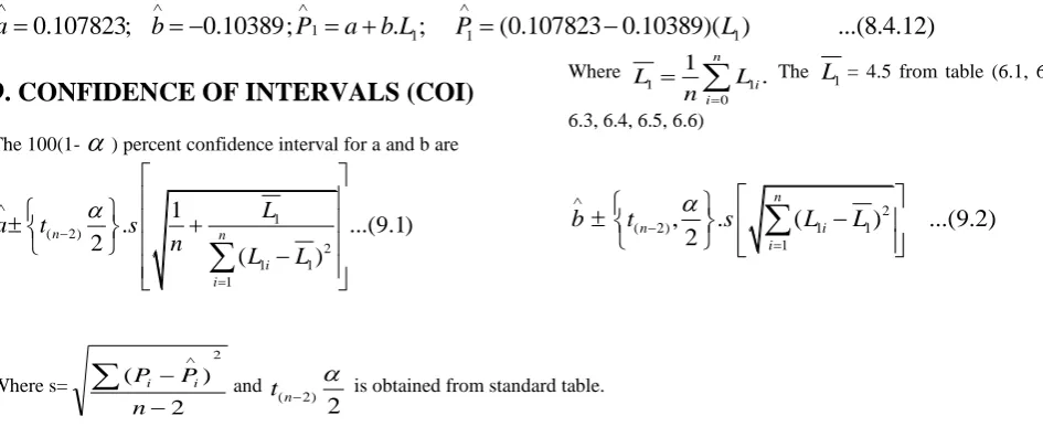
9. CONFIDENCE OF INTERVALS (COI)
The 100(1-
) percent confidence interval for a and b are1 ( 2)
2
1 1
1
1
.
...(9.1)
2
(
)
n n
i i
L
a
t
s
n
L
L
Where
1 1
0
1 .
n i i
L L
n
TheL
1= 4.5 from table (6.1, 6.2, 6.3, 6.4, 6.5, 6.6)2
( 2) 1 1
1
,
.
(
)
...(9.2)
2
n
n i
i
b
t
s
L
L
Where s=
2 ) (
2
n P
Pi i and
( 2)
2
n
t
is obtained from standard table.7
[image:8.595.58.531.75.278.2]take α=0.05,n=9 then t ,0.025=2.365
Table: 13 Confidence interval for a and b
Fixed parameter
Constant a Constant b Confidence Interval
p=0.4,L2=0.3,pA=0.2,
C1=0.3
a
=0.1690b
=-0.1622 ( a=0.16381, a=0.17435) ( b=-0.15800,b=-0.16642) p=0.6,L2=0.5,pA=0.2,C1=0.5
a
=0.403034
b
=-0.372(a=0.38117, a=0.42489 ) ( b=-0.35522, b=-0.39003) p=0.8,L2=0.7,pA=0.2,
C1=0.5
a
=0.6289
b
=-0.6060 (a=0.61121, a=0.64673) (b=-0.59188, b=-0.62018,)Average Estimates
a
0.4003
b
0.3803
1 11 1
( )
0.4003 0.3802( )
P
a
b L
P
L
Table: 14 Confidence interval for a and b
Fixed parameter
Constant a Constant b Confidence Interval
p=0.4,L2=0.3,pA=0.2,
C1=0.3
a
=0.3945b
=-0.3785 (a=0.382227, a=0.406814) (b=-0.36873,b=-0.388315) p=0.6,L2=0.5,pA=0.2,C1=0.5
a
=0.4030
b
=-0.3726(a=0.381174, a=0.424893 ) (b=-0.355201, b=-0.390025) p=0.8,L2=0.7,pA=0.2,
C1=0.5
a
=0.2695
b
=-0.2597 (a=0.261945, a=0.277171) (b=-0.25366, b=-0.26579)Average Estimates
a
0.3557
b
0.3369
1 11 1
( )
0.3557
0.3369.( )
P
a
b L
P
L
Table: 15 Confidence interval for a and b
Fixed parameter
Constant a Constant b Confidence Interval
p=0.4,L2=0.3,pA=0.2,
C1=0.3
a
=0.1183b
=-0.1135 ( a=0.114668, a=0.122044) ( b=-0.110622,b=-0.116491) p=0.6,L2=0.5,pA=0.2,C1=0.5
a
=0.2015
b
=-0.1863(a=0.190587, a=0.212447 ) ( b=-0.17761, b=-0.195011) p=0.8,L2=0.7,pA=0.2,
C1=0.7
a
=0.1886
b
=-0.1818 (a=0.183361, a=0.194019) (b=-0.17757, b=-0.18605)Average Estimates
a
0.1695
b
0.1605
1 11 1
( )
0.1695 0.1605.( )
P
a
b L
P
L
Table: 16 Confidence interval for a and b
Fixed parameter
Constant a Constant b Confidence Interval
p=0.4,L2=0.3,pA=0.2,
C1=0.2, C2=0.3
a
=0.3156
b
=-0.3028( a=0.305782, a=0.325452) (b=-0.294988,b=-0.310655) p=0.6,L2=0.5,pA=0.2,
C1=0.4, C2=0.5
a
=0.2418
b
=-0.2235(a=0.228704, a=0.254936 ) (b=-0.213122, b=-0.231022) p=0.8,L2=0.7,pA=0.2,
C1=0.6, C2=0.7
a
=0.1078
b
=-0.1038 (a=0.104778, a=0.110868) (b=-0.101477, b=-0.106322)Average Estimates
a
0.2217
b
0.2101
1 11 1
( )
0.2217
0.2101.( )
P
a
b L
P
L
10. CONCLUSION
The expression showing the simple relationships between variables
1 1
P and L, as derived by Naldi (2002) are complicated and having many input parameters like p, pA, L2
etc. If we keep all these six fixed, the expression of relationship is even not simple. By using of method least square the linear approximate relationship is displayed in table1, 2, 3, 4, 5, 6, 7, 8, 9, 10, 11 and 12. .The coefficients of determination (COD) have values near to 1 showing the best fitting of straight line between
1 1
P and L. The confidence interval for estimated value a and b are tables 13, 14, 15 and 16 indication for good fitting of line.
11. REFERENCES
[1]. Medhi, J. (1991): Stochastic models in queuing theory, Academic Press Professional, Inc., San Diego, CA. [2]. Medhi, J. (1992): Stochastic Processes, Ed.4, Wiley
Eastern Limited (Fourth reprint), New Delhi.
[3]. Chen, D.X. and Mark, J.W. (1993): A fast packet switch shared concentration and output queuing, IEEE Transactions on Networking, vol. 1, no. 1, pp. 142-151. [4]. Hambali, H. and Ramani, A. K., (2002): A performance
study of at multicast switch with different traffics, Malaysian Journal of Computer Science. Vol. 15, Issue No. 02, Pp. 34-42.
[5]. Naldi, M. (2002): Internet access traffic sharing in a multi-user environment, Computer Networks. Vol. 38, pp. 809-824.
[6]. Newby, M. and Dagg, R. (2002): Optical inspection and maintenance for stochastically deteriorating systems: average cost criteria, Jour. Ind. Statistical Associations. Vol. 40, Issue No. 02, pp. 169-198.
[7]. Francini, A. and Chiussi, F.M. (2002): Providing QoS guarantees to unicast and multicast flows in multistage packet switches, IEEE Selected Areas in Communications, vol. 20, no. 8, pp. 1589-1601.
chains and some applications, Sankhya. Vol. 66, Issue No. 02, pp. 243-252.
[9]. Paxson, Vern, (2004): Experiences with internet traffic measurement and analysis, ICSI Center for Internet Research International Computer Science Institute and Lawrence Berkeley National Laboratory.
[10]. Yeian, C. and Lygeres, J. (2005): Stabilization of class of stochastic differential equations with Markovian switching, System and Control Letters. Issue 09, pp. 819-833.
[11]. Shukla, D., Gadewar, S. and Pathak, R.K. (2007 a): A stochastic model for space division switches in computer networks, International Journal of Applied Mathematics and Computation, Elsevier Journals, Vol. 184, Issue No. 02, pp235-269.
[12]. Shukla, D. and Thakur, Sanjay, (2007 b) Crime based user analysis in internet traffic sharing under cyber crime, Proceedings of National Conference on Network Security and Management (NCSM-07), pp. 155-165, 2007.
[13]. Shukla, D., Virendra Tiwari, M. Tiwari and Sanjay Thakur [2007 c]: Rest State analysis of Internet traffic distribution in multi-operator environment published in the Journal of management Information Technology (JMIT-09), Vol. 1, pp. 72-82
[14]. Agarwal, Rinkle and Kaur, Lakhwinder (2008): On reliability analysis of fault-tolerant multistage interconnection networks, International Journal of Computer Science and Security (IJCSS) Vol. 02, Issue No. 04, pp. 1-8.
[15].Shukla, D., Tiwari, Virendra, Thakur, S. and Deshmukh, A. (2009 a):Share loss analysis of internet traffic distribution in computer networks, International Journal of Computer Science and Security (IJCSS), Malaysia, Vol. 03, issue No. 05, pp. 414-426.
[16]. Shukla, D., Tiwari, Virendra, Thakur, S. and Tiwari, M. (2009 b) :A comparison of methods for internet traffic sharing in computer network, International Journal of Advanced Networking and Applications (IJANA).Vol. 01, Issue No.03, pp.164-169.
[17]. Shukla, D., Tiwari, V. and Kareem, Abdul, (2009 c) All comparison analysis in internet traffic sharing using markov chain model in computer networks, Georgian Electronic Scientific Journal: Computer Science and Telecommunications. Vol. 06, Issue No. 23, pp. 108-115. [18]. Shukla, D, Tiwari, M., Thakur, Sanjay and Tiwari, Virendra [2009 d]: Rest State Analysis in Internet Traffic Distribution in Multi-operator Environment, (GNIM's) Research Journal of Management and Information Technology, Vol. 1, No. 1, pp. 72-82.
[19].Shukla, D. and Thakur, Sanjay [2009 e]: Modeling of Behavior of Cyber Criminals When Two Internet Operators in Markets, Accepted for publication in ACCST Research Journal, Vol. VIII, No. 3, July, (2009).
[20]. Shukla, D., Jain Saurabh, Singhai Rahul and Agarwal R.K. [2009 f]: A Markov chain model for the analysis of round robin scheduling scheme, International Journal of Advanced Networking and Applications (IJANA), vol. 01, no. 01, pp. 01-07.
[21]. Shukla, D., Thakur S. and Deshmukh Arvind [2009 g]: State probability analysis of Internet traffic sharing in computer network, International Journal of Advanced Networking and Applications (IJANA), vol. 1, issue 1, pp. 90-95.
[22]. Shukla, D., Tiwari, Virendra, and Thakur, S. (2010 a): Effects of disconnectivity analysis for congestion control in internet traffic sharing, National Conference on Research and Development Trends in ICT (RDTICT-2010), Lucknow University, Lucknow.
[23].Shukla, D., Gangele, Sharad and Verma, Kapil, (2010 b): Internet traffic sharing under multi-market situations, Published in Proceedings of 2nd National conference on Software Engineering and Information Security, Acropolis Institute of Technology and Research, Indore, MP, (Dec. 23-24,2010), pp 49-55.
[24].Shukla, D., and Thakur, S. (2010 c): Stochastic Analysis of Marketing Strategies in internet Traffic, INTERSTAT (June 2010).
[25].Shukla, D., Tiwari, V., and Thakur, S., (2010 d): Cyber Crime Analysis for Multi-dimensional Effect in Computer Network, Journal of Global Research in Computer Science(JGRCS), Vol. 01, Issue 04, pp.31-36. [26].Shukla, D., Tiwari V. and Thakur S. [2010 e]: User
behavior Based Probability Analysis of Internet Traffic Distribution in Two market in Computer Networks, Kalpagam Journal of Cambridge Studies (KJCS) [27].Shukla, D., Tiwari V. and Thakur S. [2010 f]:
Performance Analysis for Two Call Attempt of rest State Based Traffic Network, International Journal of Advanced Networking and Application (IJANA) [28].Shukla, D. and Thakur, Sanjay [2010]: Index based
Internet traffic sharing analysis of users by a Markov chain probability model. , Karpagam Journal of Computer Science, vol. 4, no. 3, pp. 1539-1545.
[29]. Shukla, D., Tiwari, V., Thakur, S. and Deshmukh, A.K. [2010 a]: Two call based analysis of internet traffic sharing, International Journal of Computer and Engineering (IJCE), Vol. 1, No. 1, pp. 14-24.
[30].Shukla, D. and Singhai, Rahul [2010 b]: Traffic analysis of message flow in three cross-bar architecture in space division switches, Karpagam Journal of Computer Science, vol. 4, no. 3, pp. 1560-1569.
[31]. Shukla, D., Thakur, Sanjay and Tiwari, Virendra [2010 c]: Stochastic modeling of Internet traffic management, International Journal of the Computer the Internet and Management, Vol. 18, no. 2 pp. 48-54.
[32]. Shukla, D., Tiwari, Virendra and Thakur, Sanjay [2010 d]: Cyber crime analysis for multi-dimensional effect in computer network, Journal of Global Research in Computer Science, Vol.1, no. 4. pp. 14-21.
[33]. Shukla, D. and Thakur, Sanjay [2010 e ]: Iso-share Analysis of Internet Traffic Sharing in Presence of Favoured Disconnectivity, GESJ: Computer Science and Telecommunications, 4(27), pp. 16-22.
Environment, Journal of Global research in Computer Science (JGRCS) Vol.2, No. 6, pp.6-12.
[35]. Shukla, D., Gangele, Sharad, Verma, Kapil and Singh, Pankaja (2011 b): Elasticities and Index Analysis of Usual Internet Browser share Problem, International Journal of Advanced Research in Computer Science (IJARCS),Vol. 02, No. 04, pp.473-478.
[36].Shukla, D., Gangele, Sharad, Verma, Kapil and Thakur, Sanjay, (2011 c): A Study on Index Based Analysis of Users of Internet Traffic Sharing in Computer Networking, World Applied Programming (WAP), Vol. 01, No. 04, pp. 278-287.
[37]. Shukla, D., Tiwari, Virendra and Thakur, Sanjay [2011] Analysis of Internet Traffic Distribution for User Behavior Based Probability in Two Market Environment, International Journal of Computer Application (IJCA), Vol. 30, Issue No. 08. pp. 44-51.
[38]. Shukla, D., Gangele, Sharad, Singhai, Rahul and Verma, Kapil, (2011 d): Elasticity Analysis of Web Browsing Behavior of Users, International Journal of Advanced Networking and Applications (IJANA), Vol. 03, No. 03, pp.1162-1168.
[39]. Shukla, D., Verma, Kapil and Gangele, Sharad, (2011 e): Re-Attempt Connectivity to Internet Analysis of User by Markov Chain Model, International Journal of Research in Computer Application and Management (IJRCM) Vol. 01, Issue No. 09, pp. 94-99.
[40]. Shukla, D., Gangele, Sharad, Verma, Kapil and Trivedi, Manish, (2011 f): Elasticity variation under Rest State Environment In case of Internet Traffic Sharing in Computer Network, International Journal of Computer Technology and Application (IJCTA) Vol. 02, Issue No. 06, pp. 2052-2060.
[41]. Shukla, D., Gangele, Sharad, Verma, Kapil and Trivedi, Manish, [2011]: Two-Call Based Cyber Crime Elasticity Analysis of Internet Traffic Sharing In Computer Network, International Journal of Computer Application (IJCA) Vol.02, Issue 01, pp.27-38.
[42]. Shukla, D., Singhai, Rahul [2011]: Analysis of User Web Browsing Using Markov chain Model, International Journal of Advanced Networking and Application (IJANA), Vol. 02, Issue No. 05, pp. 824-830.
[43]. Shukla, D., Verma, Kapil and Gangele, Sharad, [2012]: Iso-Failure in Web Browsing using Markov Chain Model and Curve Fitting Analysis, International Journal of Modern Engineering Research(IJMER) , Vol. 02, Issue 02, pp. 512-517.
[44]. Shukla, D., Verma, Kapil and Gangele, Sharad, [2012]: ]: Least Square Curve Fitting in Internet Access Traffic Sharing in Two Operator Environment, International Journal of Computer Application (IJCA), Vol.43(12), pp. 26-32.
[45]. Shukla, D., Verma, Kapil and Gangele, Sharad, [2012]: Curve Fitting Approximation in internet traffic Distribution in computer network in two Market Environment, International Journal of Computer Science and Information Security, (IJCSIS), Vol. 10, Issue 04, pp 71-78.