Comparison between H
∞
and CRONE Control Combined
with QFT Approach to Control Multivariable Systems in
Path Tracking Design
Najah Yousfi
1, Pierre Melchior
2, Chokri Rekik
1, Nabil Derbel
1, Alain Oustaloup
21 Control & Energy Management laboratory (CEM), University of Sfax, Sfax Engineering School, BP W, 3038 Sfax, Tunisia.
2 IMS (UMR 5218 CNRS, Université Bordeaux 1 - ENSEIRB - ENSCPB), Département LAPS 351 cours de la Libération, Bât. A4 - F33405 TALENCE cedex, France.
ABSTRACT
Motion control and robust path tracking were the subject of this paper. A method based on fractional prefilter which is extended to multivariable systems is developed. This approach is based on the MIMO-QFT robust synthesis methodology combined with CRONE control. This paper incorporates Quantitative Feedback Theory (QFT) principles to CRONE control design procedure to solve the Two-Degree-Of-Freedom (TDOF) with Highly Uncertain Plants. A comparison between H∞ and CRONE controllers has been
done. After that, synthesis of fractional prefilters is given with optimization of its parameters using integral gap criterion. To assess the proposed design, a numerical example has been considered.
General Terms
Path tracking design using CRONE control approach applied to multivariable systems.
Keywords
Path tracking, MIMO structures, H∞ design, CRONE control,
Robotics.
1.
INTRODUCTION
One of the most painful problems is the MIMO (Multiple- Input-Multiple-Output) control of uncertain systems. Many approach treated the robust generation of tracking trajectory. The fractional differentiation approach [1], [2] applied to non time-varying plants has been developed. According to only two parameters (n, τ) this method can permits to generate profiles of position, speed and acceleration. These profiles can be obtained by considering the physical limitation of actuators and control frequency bandwidth [1], [3]. This approach has been extended to multivariable systems using MIMO-QFT robust synthesis methodology [4].
The Quantitative Feedback Theory (QFT) design was introduced by Horowitz [5], [6], [7], [8]. The general problem in the QFT Two Degree Of Freedom (TDOF) system is how to generate the feedback controller and the prefilter [9]. Specifications of most QFT problems are to put the responses of the closed loop system into lower and upper bounds [9], [10]. QFT design techniques have been developed for highly uncertain linear time invariant MIMO single-loop matrix and multiple-loop matrix systems [7], [11], [12].
The CRONE control-system design which is introduced by Oustaloup et al. [14], [17] is based on fractional non-integer differentiation [16], [18]. The Crone control is a frequency design to provide the robust control of perturbed plants using the common unity feedback configuration. For the nominal state of the plant, this approach consists on determining the
open-loop transfer function which guarantees the desired specifications like precision, overshoot and rapidity. The controller can be obtained from the ratio of the open loop transfer function to the nominal plant transfer function taking into account the plant right half-plane zeros and poles. There are three CRONE control generations [15], [19]. Only the used principle of the third generation is given in this paper. The fractional non-integer differentiation allows to describe the open-loop transfer function. The optimal transfer function to meet the specifications is easier to obtain. Furthermore, instead of H∞ procedures the CRONE control design takes
into account the plant genuine structured uncertainty domains. CRONE control design has already been applied to multivariable systems [15], [20]
The objective of this paper is to extend the CRONE control approach to multivariable systems using fractional prefilters in path tracking design. A comparison between QFT/H∞ and QFT/CRONE designs with fractional prefilter is used to resolve the problem of square multivariable systems. The QFT/H∞ and QFT/CRONE synthesis procedures are used for each SISO loop. Then the SISO fractional prefilter is developed after optimization based on physical constraints and tracking specifications.
Section 2, summarizes the MIMO-QFT procedure. The H∞ control is presented in section 3. Section 4 gives the CRONE control approach for multivariable plants. Section 5 deals with fractional prefilter optimization. The result of simulations is presented by 2 × 2 uncertain MIMO plant in section 6.
2.
MIMO-QFT STRUCTURE:
Fig.1 gives the MIMO QFT structure:
Fig 1 Two-degrees-of-freedom control system : MIMO structure
𝑃 = 𝑝𝑖𝑗 𝑚×𝑚 is a given 𝑚 × 𝑚 plant transfer function matrix. P represents the linear time invariant uncertain plant to be controlled
.
𝑃
should be square and minimum-phase. The controller 𝐺 𝑝 = 𝑑𝑖𝑎𝑔 𝑔𝑖𝑖 reduces the uncertainties effects and the prefilter matrix F(p) leaves the response into the desired region.The transfer matrix is given by (see fig1):
P, the plant transfer function matrix, must be nonsingular, so: [𝑃−1+ 𝐺]𝑇 = 𝐺𝐹 (2) P-1, the inverse matrix, is decomposed to this form:
𝑃−1= 𝛬 + 𝐵 (3) where 𝛬 is the diagonal part, and B is the anti-diagonal part of P−1.
Elements of matrix Q are expressed by: 𝑞𝑖𝑗=𝑎𝑑𝑗 (𝑃det (𝑃)
𝑖𝑗) (4) Considering into account (3), equation (2) can be transformed to this form:
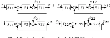
[image:2.595.56.284.328.407.2]𝑇 = [𝛬 + 𝐺]−1[𝐺𝐹 − 𝐵𝑇] (5) For a square MIMO system, a 2×2 system is equivalent to a 4 subsystems (MISO structure) which is proved by Horowitz [5], [17] (see figure 2) :
Fig 2 Equivalent diagram for 2x2 MIMO system
Elements of the transfer matrix T have the following form: 𝑡𝑖𝑗= 𝜔𝑖𝑖 𝜈𝑖𝑗+ 𝑑𝑖𝑗 = 𝑡𝑟𝑖𝑗+ 𝑡𝑑𝑖𝑗 (6) where:
𝜔𝑖𝑖 =1+𝑔𝑞𝑖𝑖
𝑖𝑞𝑖𝑖 𝜈𝑖𝑗 = 𝑔𝑖𝑓𝑖𝑗 and
𝑑𝑖𝑗 = −
𝑡𝑘𝑗
𝑞𝑖𝑘 , 𝑘 = 1,2, … , 𝑚 𝑚
𝑘≠𝑖
The MISO system design becomes SISO-QFT design when dij appears as “disturbance” [1]. The aim of this technique is to allow each loop track its desired input while minimizing outputs caused by disturbance inputs [1]. To reject disturbances, there is a given limit to the responses tdij [18]. Let a small real positive function σij(ω) such that:
1+𝑞 1
𝑖𝑖 𝑗𝜔 𝑔𝑖(𝑗𝜔 ) ≤
𝜎𝑖𝑗 (𝜔)
−𝑞𝑖𝑖(𝑗𝜔 )/𝑞𝑖𝑗(𝑗𝜔 ) (7)
𝑖 ≠ 𝑗, 𝑗 = 1,2, …,
3.
𝑯
∞𝑪𝑶𝑵𝑻𝑹𝑶𝑳
To achieve robust performances, H∞ design can be used to synthesis controllers. The most important problem of H∞
control design is how to move selection of the weighting
functions so that the control loop satisfies all design requirements.
The first step of the feedback system design is the weight selection of different functions (see (8))
𝑊𝑠 𝑗𝜔 𝑆(𝑗𝜔) ∞< 1
𝑊1 𝑗𝜔 𝑇1(𝑗𝜔) ∞< 1
𝑊𝑢𝑛 𝑗𝜔 𝑇𝑢𝑛(𝑗𝜔) ∞< 1
(8)
where 𝑇𝑢𝑛 𝑝 = 𝐺 𝑝 𝑆 𝑝 is the transfer function related to the amplification of the sensor noise, 𝑇1= 𝐼 + 𝑃𝐺 −1𝑃𝐺 is the complementary sensitivity function and 𝑆 = 𝐼 + 𝑃𝐺 −1 is the sensitivity function.
The standard 𝐻∞optimal regulator problem initially described by Skogestad and Postelewaite [12] is called the mixed sensitivity problem. Taking into consideration the following relations, the structure in Fig.3b can be derived from the feedback control setup of Fig.3a:
𝑍1 𝑝 = −𝐺 𝑝 𝑆 𝑝 𝑊𝑢𝑛 𝑝 𝑛 𝑝 = 𝑇𝑢𝑛𝑊𝑢𝑛𝑛(𝑝)
𝑍2 𝑝 = 𝑇1(𝑝)𝑊𝑀𝑃 𝑝 𝑟1 𝑝 = 𝑇𝑢𝑓𝑊𝑀𝑃𝑟(𝑝)
𝑍3 𝑝 = 𝑆 𝑝 𝑊𝑠 𝑝 𝑑 𝑝
(9)
These equations (9) can leads to obtain the generalized plant
Paug. So, to have a more general interpretation than only the mixed sensitivity problem, the structure in Fig.3a can be presented by Fig.3b. This presentation in Fig.3b is used for any MIMO control feedback system.
The generalized plant Paug is an augmented plant where W(p) is the external inputs (like d, n and r (see Fig.3a)), u is the controlled input, z is a vector of weighted external outputs, and e is the error delivered to the controller G(p).
Fig 3 Mixed sensitivity standard problem
After choosing the nominal plant and different weighting functions WMP, Wun and Ws, the controller G(p) can be calculated using hinsyn from µ− Analysis and Synthesis Toolbox of Matlab.
4.
CRONE CONTROL
[image:2.595.321.539.420.502.2]β0 p =
β01 p ⋯ 0
⋮ ⋱ ⋮
0 ⋯ β0n p
(10)
The nominal sensitivity 𝑆0(𝑝) the nominal complementary sensitivity 𝑇0(𝑝), input sensitivity 𝑆𝑈0(𝑝) and input disturbance sensitivity 𝑆𝑙0(𝑝) transfer function matrices are :
S0 p = I + β0 p −1= diag S0j p 1≤j≤n (11)
T0 p = I + β0 p −1β0 p = diag T0j p 1≤j≤n (12)
SU0 p = G(p) I + β0 p −1= G(p) S0 p (13)
Sl0 p = I + β0 p −1Q(p) = T0 p G−1(p) (14) With:
T0j p =1+ββ0 p 0 p (15)
S0j p =1+β1
0 p (16) The open-loop transfer functions β0i p are used to satisfy some objectives:
accuracy specifications at low frequencies,
required nominal stability margins of the closed-loops
specifications on the n control efforts at high frequencies.
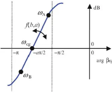
[image:3.595.76.260.494.649.2]The third generation of CRONE CSD uses complex non integer order integration over a selected frequency range 𝜔𝐴 , 𝜔𝐵 . The generalized template is a straight line of any direction in the Nichols chart created by the complex fractional order 𝑛𝑓= 𝑎 + 𝑖𝑏 (fig 4):
Fig 4 The generalized template
Its phase location at frequency 𝜔𝑐𝑔 is given by the real part of
𝑛𝑓and the imaginary part defines its direction [23]. When the generalized template is based on band-limited complex non
integer integration, then the transfer function is [24], [26]:
β0i p = Csign (b) 1+p/ω1+p/ωh l
a
×
Re/i Cg1+p/ω1+p/ωh l
ib
−qsign (b)
(17)
C = ch b arctan ωωcg l −
ωcg
ωh (18)
Cg= 1+ ω cg
ω l 2
1+ ω cg ω h 2
1/2
(19)
The corner frequencies are placed such that: ωl< ωA< ωcg < ωB< ωh (20) In the open-loop transfer function, the generalized template is taken into account when the plant is stable and minimum phase:
β0ii p = βli p β0i p βhi p (21) where
βli p = Cli ωpli− 1 nli
(22)
βhi p = p Cli ω hi+1
n hi (23)
The accuracy of each closed-loop is fixed by the order 𝑛𝑙𝑖but the order 𝑛𝑖allows the elements of the controller to be proper.
Consider that Q0 is the nominal plant transfer matrix such that Q0 p = q0ij(p) i,j∈N:
β0= Q0G = diag β0i i=j= diag ndi
i i∈N (24) where:
β0i=ndi
i , the element of the i
th
column and row.
The objective of CRONE control for MIMO plants is to determine a decoupling controller for the nominal plant. Q0 being not diagonal, the problem is to find a decoupling and stabilizing controller G. The controller exists if the following hypotheses are true [24]:
H1: Q(p) −1 exists, (25) H2: Z+[Q p ] ∩P+ Q p = 0 (26) where Z+[Q p ] and P+[Q p ] are respectively the positive
real part zero and pole sets.
The controller G is described by:
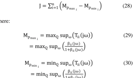
For each nominal open-loop β0(p), many generalized templates can border the same required magnitude-contour of the Nichols chart or the same resonant peak Mp0i. The optimal
one minimizes the robustness cost function:
J = ni=1 Mpmax i− Mpmin i (28)
where: Mpmax i = maxQsupω Tii jω (29)
= maxQsupω 1+ββii(jω) ii(jω) Mpmin i = minQsupω Tii jω (30)
= minQsupω 1+ββii jω ii jω This optimization can be done while respecting the following set for ωϵR and i, jϵN : infQ Tij jω ≥ Tijl ω (31)
supQ Tij jω ≥ Tiju ω (32)
supQ Sij jω ≥ Siju ω (33)
supQ GSij jω ≥ G Siju ω (34)
supQ Sij jω ≥ SQiju ω (35)
where Q is the nominal or perturbed plant. A non-linear optimization method permits the extraction of the independent parameters of each open loop transfer function. Respecting other specifications taken into account by constraints on sensitivity function magnitude, this optimization is based on minimization of the stability degree variations.
5.
FRACTIONAL PREFILTER
OPTIMIZATION
Bang-Bang laws and Polynomial interpolation approaches have a bandwidth that varies with the length of the displacement. Owing to these variations, we can observe overshoots for small displacements. Optimization in the frequency domain for all displacements in order to limit end actuator vibration is obtained by digital filters that have a fixed bandwidth. A low-pass filter is described by the transmittance:F p = 1+τp 1 n = 1 1+ωp n (36) [image:4.595.316.526.76.344.2]
which uses real poles and prevents frequency resonance. The choice of identical poles can leads to the largest possible energy on bandwidth (Fig.5(a)). Davidson-Cole prefilter [28] (see (36)), at high frequencies, reduces energy of the signal. As can be seen in Fig.5(b), it continuously controls the bandwidth (time constant τ) and the selectivity (real order n). As analog or digital filter, it can be used as prefilter to reduce overshoots in position control. Fig 5 (a) : Pole assignment for a maximum energy in a given pass band; (b) : Frequency response of the Davidson-Cole filter Considering Fig.6, the reference sensitivity transfer function Sref between control u and input r is given by: Sref p = F p G(p) 1+G p Q(p) (37)
Fig 6 Unity feedback control loop with prefilter In order to keep the control signals under its maximum value, the frequency constraint is: ∀ ω > 0, 𝜏 > 0, Sref jω ≤ γ (38)
where γ =uemax max , with umax the maximum static constraint value on the control signal and emaxis a constant signal to apply on the prefilter input. The desired range of the closed-loop transfer function is described by two bounds in frequency domain which are detailed bellow: ∀ ω > 0, 𝜏 > 0, TRL jω ≤ trii jω ≤ TRU jω (39)
This equation becomes: ∀ ω > 0, 𝜏 > 0, TRL jω ≤ trii jω min (40)
trii jω max ≤ TRU jω (41)
[image:4.595.62.278.129.255.2]By considering the integral gap criterion, we can obtain the optimized parameters of the Davidson-Cole filter can be obtained. The integral gap analytic expression for step response is:
Ie≤ nτ (43)
For m × m MIMO systems, the integral gap criterion is calculated as MISO sub-system [1], so in the case of F =diag[fii] the Eq.(43) becomes:
Ie≤ n1τ1+ n2τ2+ ⋯ + nmτm (44)
We can find the optimal parameters of (n, τ) using the optimization toolbox of MATLAB.
6.
APPLICATION
The proposed control design will be illustrated in this part. There is a given 2 × 2 uncertain MIMO plant with transfer function:
𝑃 𝑝 = 𝑝𝑝11 𝑝12
21 𝑝22 (45) 𝑝𝑖𝑗 𝑝 =
𝑘𝑖𝑗
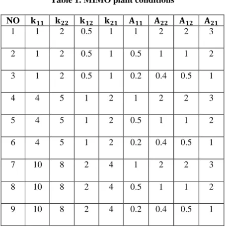
1+𝐴𝑖𝑗𝑝 (46) 9 plant cases are given in table 1.
The tracking specification of the closed loop transfer function are enforced to be into the following upper and lower bounds:
𝑇𝑅𝑈𝑖𝑖 𝑝 =
0.08𝑝2+3𝑝+25
0.002𝑝3+1.015𝑝2+7.55𝑝+25 (47)
𝑇𝑅𝑈𝑖𝑖 𝑝 =
96
𝑝4+18.5𝑝3+105.5𝑝2+184𝑝+96 (48)
6.1
𝑯
∞controller
After selection of weighting function which is the objective of another paper, the suitable controller is described by:
𝐺𝐻∞ 𝑝 = 𝐺11𝐻0∞(𝑝) 𝐺 0
22𝐻∞(𝑝) (49)
where
𝐺11𝐻∞ 𝑝 = 𝑝+1.471𝑒6 𝑝+6.127 (𝑝+0.01)8540766 .6956 𝑝+5 (𝑝+1.09)
𝐺22𝐻∞ 𝑝 = 94811.6956 𝑝+2.5 (𝑝+1.09) 𝑝+4033 𝑝+3.685 (𝑝+0.01)
To synthesis the fractional prefilter, the first and ninth plants are respectively represents the maximum and minimum plant. Secondly, the ratio 𝑢𝑒𝑚𝑎𝑥
𝑚𝑎𝑥 = 1 is fixed. By minimizing the integral gap criterion (44), optimized parameters are obtained with m = 2 respecting the frequency bound inequality (38) and the performance specifications (39):
𝑛1= 1.5001, 𝜏1 = 0.2001 (50)
[image:5.595.315.543.88.320.2]𝑛2= 1.3458, 𝜏2= 0.4356 (51)
Table 1. MIMO plant conditions
NO 𝐤𝟏𝟏 𝐤𝟐𝟐 𝐤𝟏𝟐 𝐤𝟐𝟏 𝐀𝟏𝟏 𝐀𝟐𝟐 𝐀𝟏𝟐 𝐀𝟐𝟏
1 1 2 0.5 1 1 2 2 3
2 1 2 0.5 1 0.5 1 1 2
3 1 2 0.5 1 0.2 0.4 0.5 1
4 4 5 1 2 1 2 2 3
5 4 5 1 2 0.5 1 1 2
6 4 5 1 2 0.2 0.4 0.5 1
7 10 8 2 4 1 2 2 3
8 10 8 2 4 0.5 1 1 2
9 10 8 2 4 0.2 0.4 0.5 1
The approximation of these fractional prefilters to the integer order has been developed using the module “Frequency Domain System Identification” of the CRONE toolbox [28] in MATLAB environment.
𝐹𝐷𝐶𝐻 𝑝 = 𝐹1𝐷𝐶𝐻0 𝐹0
2𝐷𝐶𝐻 (52)
𝐹1𝐷𝐶𝐻 𝑝 = 𝑝+77.93 𝑝+55.44 𝑝+46.4 𝑝+4.471 (𝑝+9.735)0.71937 𝑝+97.95 𝑝+87.19 𝑝+71.07 (𝑝+19.98)
𝐹2𝐷𝐶𝐻 𝑝 =
0.42222 𝑝+96.75 𝑝+65.98 𝑝+21.63 (𝑝+9.693)(𝑝+5.248)
𝑝+70.33 𝑝+35.29 𝑝+20.41 𝑝+7.096 (𝑝+2.901)(𝑝+2.84)
6.2
𝑪𝑹𝑶𝑵𝑬
controller
The first plant is considered as the nominal case. The following specifications must be satisfied for all plants:
For both outputs zero steady-state error
Settling time as short as possible
Robustness according to disturbances and parametric variations
A first overshoot less than 5%.
Some elements of the open-loop transfer function matrix can be initialized while considering these specifications. With all these specifications, the initial values for the parameters of the first fractional open-loop transfer function are:
𝜔𝑟1= 19.5587 𝑟𝑎𝑑/𝑠
𝜔𝑙1= 3.93722 𝑟𝑎𝑑/𝑠
𝜔1= 36.7678 𝑟𝑎𝑑/𝑠
𝛽01(𝑗𝜔) 𝜔=𝜔𝑟1= 0.66303 𝑑𝐵
𝑛𝑙 = 1
𝑛 = 2
And for the second
𝜔𝑟2= 30.1265 𝑟𝑎𝑑/𝑠
𝜔𝑙2= 46.8651 𝑟𝑎𝑑/𝑠
𝜔2= 415.181 𝑟𝑎𝑑/𝑠
𝛽02(𝑗𝜔) 𝜔=𝜔𝑟2= 6.19809 𝑑𝐵
𝑛𝑙 = 1
Taking into account all the specifications, the optimal values for the various parameters of open loop transfer function matrix are:
For the first loop: 𝐶1. 𝐶𝑙1= 5.43596, 𝑎11.02996,
𝑏1= −0.648348, 𝑞1= 1 and 𝐶1= 4.4737
For the second loop: 𝐶2. 𝐶𝑙2= 1.44976, 𝑎2=
1.46743, 𝑏2= 0.375524, 𝑞2= 1 and 𝐶2= 1.18568 The controller expression while respecting all these specifications is:
𝐺𝑐𝑟𝑜𝑛𝑒 𝑝 = 𝐺11𝑐𝑟𝑜𝑛𝑒0 (𝑝) 𝐺 0
22𝑐𝑟𝑜𝑛𝑒(𝑝) (53) with
𝐺11𝑐𝑟𝑜𝑛𝑒 𝑝 =1180.9191 𝑝+2.96 (𝑝+0.951)𝑝 𝑝+22.5 (𝑝+6.84)
𝐺22𝑐𝑟𝑜𝑛𝑒 𝑝 =
1260.0602 𝑝+3476 (𝑝+844.9)(𝑝+111)(𝑝+78.79)(𝑝+0.5) 𝑝 𝑝+785 𝑝+579 (𝑝+246)(𝑝+90.6)(𝑝+52.2)
The prefilter synthesis is as described in section 6.1, so the optimized parameters are obtained by minimization of integral gap criterion and under frequency constraints:
𝑛1= 1.5, 𝜏1= 0.18814 (54)
𝑛2= 1.4046, 𝜏2= 0.2075 (55)
The integer order approximation of the fractional prefilter
FDCC is determined by using the module “Frequency Domain System Identification” of the CRONE software [27]:
𝐹𝐷𝐶𝐶 𝑝 = 𝐹1𝐷𝐶𝐶0(𝑝) 𝐹 0
2𝐷𝐶𝐶(𝑝) (54) with
𝐹1𝐷𝐶𝐶(𝑝) =
0.23259 𝑝+966.8 (𝑝+830.8)(𝑝+79.19)(𝑝2+621.7𝑝+9.664𝑒4) 𝑝+546.1 (𝑝+463.3)(𝑝+18.99)(𝑝+3.899)(𝑝2+550.3𝑝+7.629𝑒4)
𝐹2𝐷𝐶𝐶(𝑝) =0.34617 𝑝+958.4 (𝑝+815.4)(𝑝+265.4)(𝑝+165.9)(𝑝+16.5) 𝑝+640 (𝑝+415.4)(𝑝+299.7)(𝑝+72.3)(𝑝2+11.68𝑝+34.1)
The resultant time domain closed-loop tracking response under all nine operating conditions is illustrated using fractional prefilters and a classical prefilter Fcl in Fig.7. The classical prefilter is described by the following expression:
𝐹𝑐𝑙 𝑝 = 𝐹𝑐𝑙10(𝑝) 𝐹 0
𝑐𝑙2(𝑝) (57) where
𝐹𝑐𝑙1=𝑝+11 , 𝐹𝑐𝑙2=𝑝+1.51.5
Under all nine operating plant cases, the time domain closed-loop tracking responses are illustrated. All plants respect the desired specifications shown by upper and lower bound. A comparison of the found results with thus of the closed-loop tracking responses obtained with a classical pre-filters Fcl shows the benefit of using fractional prefilters. The fractional prefilter gives faster responses in time domain (Fig.7).
(a)
(b)
Fig 7 (a), (b) :Closed loop tracking response with classical (red) and fractional prefilters (green), tracking references
(blue)
6.3
Comparison of two type of controllers
Using both H∞ and CRONE controllers with the fractional
prefilters (Eq.(49), (52), (53) and (56)), the time domain responses are clarified in Fig.8:
(a)
0 1 2 3 4 5 6 7
0 0.2 0.4 0.6 0.8 1
Step Response
Time (sec)
A
m
p
lit
u
d
e
0 1 2 3 4 5 6 7
0 0.2 0.4 0.6 0.8 1
Step Response
Time (sec)
A
m
p
lit
u
d
e
0 1 2 3 4 5 6 7
0 0.2 0.4 0.6 0.8 1
Step Response
Time (sec)
A
m
p
lit
u
d
[image:6.595.328.522.85.430.2](b)
Fig 8 (a), (b) : Closed loop tracking response with H (red) and CRONE controllers (green), tracking references
[image:7.595.74.261.85.250.2](blue)
Table 2. Comparison between H∞and CRONE controllers
using the first
Settling time (s) Rise time (s) Controller 𝑃11 𝑃22 𝑃11 𝑃22
H∞ 1.24 1.48 0.843 1.077
CRONE 0.942 0.772 0.637 0.552 Table.2 gives the settling time and the rise time for the first case plant using different types of controllers (H∞ and
CRONE). The comparison shows that the CRONE controller gives the most performant responses. The settling time has been ameliorated and it was practically the half of the settling time obtained by the H∞ controller. So, the CRONE controller can gives the most rapid responses.
7.
CONCLUSION
A path tracking design based on fractional prefilters has been extended to multivariable approach using CRONE methodology. The parallelism between QFT design and fractional prefilter has been developed with both H∞ and CRONE controller. The simulation on a 2×2 uncertain MIMO system shows that CRONE control approach successfully states the robust stability of the closed-loops, the robust decoupling and the robust disturbances rejection. Using classical and fractional prefilters, it’s clear that the use of Davidson Cole filters is efficient. The comparison between the two types H∞ and CRONE controllers using fractional prefilters has been shown.
8.
REFERENCES
[1] P. Melchior, B. Orsoni, Th. Badie, G. Robin. Génération de consigne optimale par filtre à dérivée généralisée implicite : Application au véhicule électrique. In Proceedings of the IEEE CIFA’2000 conference, Lille, France, 2000.
[2] A. Poty, P. Melchior, A. Oustaloup. Frequency band-limited fractional differentiator in path tracking design. In Proceedings of the second IFAC Workshop on Fractional Differentiation and its Applications, Portugal, 2006.
[3] P. Melchior, G. Robin, S. L’Hostis, F. Levron. Non integer order movement generation in path planning. In
Proceedings of IEEE-SMC CESA 98 IMACS, Nabeul Hammamet, Tunisia, 4:371-375, April 1-4, 1998. [4] P. Melchior, C. Inarn, A. Oustaloup. Path tracking design
by fractional prefilter extension to square MIMO systems. In Proceedings of the ASME 2009 International Design Engineering Technical Conferences and Computers and Information in Engineering Conference, California, USA, 2009.
[5] I. Horowitz. Synthesis of Feedback Systems. Academic Press, New York, 1963.
[6] I. Horowitz. Quantitative synthesis of uncertain multiple input- output feedback system. International Journal of Control, 30(1), 81-106, 1979.
[7] I. Horowitz. Survey of quantitative feedback theory (QFT). International Journal of Robust and Nonlinear Control, 11, 887-921, 2001.
[8] I. Horowitz, M. Sidi. Synthesis of feedback systems for prescribed time domain tolerances. International Journal of Control, 16(2), 287-309, 1972.
[9] S. Mohammad, M. Alavi, A. Khaki Sedigh, B. Labibi. Pre-Filter design for tracking error specifications in MIMO-QFT. In Proceeding of the 44th IEEE Conference on Decision and Control, and the European Control Conference, Seville, Spain, 2005.
[10] E. Boje. Non-diagonal controllers in MIMO quantitative feedback design. International Journal of Robust and Nonlinear Control, 2002.
[11] W. Zenghui, C. Zengqiang, S. Qinglin, Y. Zhuzh. Multivariable decoupling predictive control based on QFT theory and application in CSTR chemical process. Chinese J. Chem. Eng, 2006.
[12] S. Skogestad, I. Postlethwaite. Multivariable feedback control, Analysis and design. JHON WILEY & SONS, New York, 1996.
[13] C.C. Cheng, Y.K. Liao, T.S. Wang. Quantitative feedback design of uncertain multivariable control system. International Journal of Control, 65(3), 537-553, 1996.
[14] A. Oustaloup. Fractional order sinusoidal oscillators: optimization and their use in highly linear F.M. modulation. IEEE Transactions on Circuits and Systems, 28(10), 1007- 1009, 1981.
[15] A.Oustaloup, B. Mathieu. La commande CRONE: Du scalaire au multivariable. Hermès Editions, Paris, 1999. [16] A. Oustaloup, B. Mathieu, P. Lanusse. Intégration non
entière complexe et contours d’isoamortissement. Automatique, Productique, Informatique Industrielle 29(1), 177-202, 1995.
[17] A. Oustaloup. The CRONE control. In Proceedings of the European Control Conference ECC’91, Grenoble, France, July, 1991.
[18] P. Lanusse. De la commande CRONE de première génération à la commande CRONE de troisième génération. PhD thesis, Bordeaux I University, France, 1994.
[19] A. Oustaloup, B. Mathieu, P. Lanusse, J. Sabatier. La commande CRONE. 2nd
edition. Editions HERMES, Paris, 1999.
[20] P. Lanusse, D. Nelson Gruel, J. Sabatier, R.Lasnier et A. Oustaloup. Synthèse multivariable d’une commande
0 1 2 3 4 5 6 7
0 0.2 0.4 0.6 0.8 1
Step Response
Time (sec)
A
m
p
lit
u
d
[image:7.595.75.260.334.381.2]CRONE décentralisée. Automatique et Informatique Appliquée, éditions de l’Académie Roumaine, 2009. [21] A. Oustaloup, B. Mathieu, P. Lanusse. The CRONE
control of resonant plants: application to a flexible transmission. Eur. J. Control, 1(2), 1995.
[22] P. Lanusse, A. Oustaloup, B. Mathieu. Robust control of LTI square MIMO plants using two CRONE control design approaches. IFAC Symposium on Robust Control Design ROCOND 2000, Prague, Czech Republic, 2000. [23] CRONE research group. CRONE control design module
user’s guide. Version 4.0, 2010.
[24] D. Nelson Gruel, P. Lanusse, A. Oustaloup. Decentralized CRONE control of m × n multivariable system with time-delay. Springer Book entitled “New Trends in Nanotechnology and Fractional Calculus Applications”, 2009.
[25] Y. JANAT. Commande CRONE monovariable et multivariable de systèmes peu amortis. PhD thesis, Bordeaux I University, France, 2007.
[26] D. Nelson Gruel, P. Lanusse, A. Oustaloup. Robust control design for multivariable plants with time-delays. Chemical Engineering Journal, 146, 414-427, 2009. [27] A. Oustaloup , P. Melchior, P. Lanusse , O. Cois , F.
Dancla. The CRONE toolbox for Matlab. In Proceeding of the IEEE Int. Symp. on Computer-Aided Control-System Design, Anchorage, USA, 2000.